Derivation
The Maxwell–Boltzmann (MB) distribution  describes the velocities
 or the kinetic energy
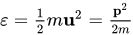 of the particles at thermal equilibrium, far from the limit of the speed of light, i.e.:
 | | 1 |
where the low-energy limit (non-relativistic) can be expressed as  , or equivalently,
 . Here,
 is the expression of temperature as a speed, called thermal speed, and n denotes the kinetic degrees of freedom of each particle. (Note that the temperature is defined in the fluid's rest frame, where the bulk speed
 is zero. In the non-relativistic case, this can be shown by using
 .
The relativistic generalization of Eq. (1), that is, the Maxwell–Jüttner (MJ) distribution, is given by:
 | | 2 |
where 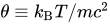 ,
 , and
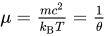
 . (Note that the inverse of the unitless temperature
 is the relativistic coldness
 .[6]) This distribution (Eq. 2) can be derived as follows. According to the relativistic formalism for the particle momentum and energy, one has

While the kinetic energy is given by  . The Boltzmann distribution of a Hamiltonian is
 . In the absence of a potential energy,
 is simply given by the particle energy
 , thus:

(Note that is the sum of the kinetic  and rest energy
 ,
 ). Then, when one includes the n-dimensional density of states:

So that:

Where  denotes the n-dimensional solid angle. For isotropic distributions, one has

or

Then,  so that:
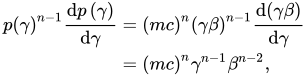
Or:
 | | 3 |
Now, because  . Then, one normalises the distribution Eq. (3). One sets

And the angular integration:

Where  is the surface of the unit n-dimensional sphere. Then, using the identity
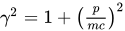 one has:
;\theta )\,\mathrm {d} p_{1}\cdots \mathrm {d} p_{n}={\frac {N}{2}}B_{n}\left(mc\right)^{n}\,e^{-\gamma /\theta }\left(\gamma ^{2}-1\right)^{{\frac {n}{2}}-1}\,\mathrm {d} (\gamma ^{2}-1).}
 and
;\theta )\,\mathrm {d} p_{1}\cdots \mathrm {d} p_{n}\\[1ex]&={\frac {N}{2}}B_{n}\left(mc\right)^{n}\,\int _{1}^{\infty }e^{-{\frac {\gamma }{\theta }}}\left(\gamma ^{2}-1\right)^{{\frac {n}{2}}-1}\mathrm {d} (\gamma ^{2}-1)\\[1ex]&={\frac {N}{2}}B_{n}\left({\frac {n}{2}}\right)^{-1}\left(mc\right)^{n}\theta ^{-1}\,\int _{1}^{\infty }e^{\frac {\gamma }{\theta }}\left(\gamma ^{2}-1\right)^{\frac {n}{2}}\mathrm {d} \gamma \\[1ex]&={\frac {N}{2}}B_{n}\left({\frac {n}{2}}\right)^{-1}\left(mc\right)^{n}\theta ^{-1}\,I_{n},\end{aligned}}}
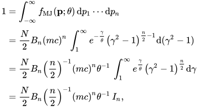
Where one has defined the integral:

The Macdonald function (Modified Bessel function of the second kind) (Abramowitz and Stegun, 1972, p.376) is defined by:

So that, by setting 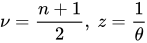 one obtains:

Hence,
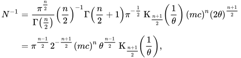
Or

The inverse of the normalization constant gives the partition function  :

Therefore, the normalized distribution is:

Or one may derive the normalised distribution in terms of:
;\theta )\,\mathrm {d} \gamma ={\frac {\pi ^{\frac {1}{2}}2^{\frac {1-n}{2}}}{\Gamma {\left({\frac {n}{2}}\right)}}}\theta ^{\frac {1-n}{2}}{\frac {e^{-\gamma /\theta }}{\operatorname {K} _{\frac {n+1}{2}}{\!\!\left({\frac {1}{\theta }}\right)}}}\left(\gamma ^{2}-1\right)^{{\frac {n}{2}}-1}\gamma \,\mathrm {d} \gamma }

Note that can be shown to coincide with the thermodynamic definition of temperature.
Also useful is the expression of the distribution in the velocity space.[7] Given that  , one has:
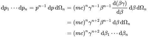
Hence
;\theta )\,\mathrm {d} \beta _{1}\cdots \mathrm {d} \beta _{n}=\pi ^{\frac {1-n}{2}}2^{-{\frac {n+1}{2}}}\,\theta ^{\frac {1-n}{2}}{\frac {e^{-\gamma (\beta )/\theta }}{\operatorname {K} _{\frac {n+1}{2}}{\!\!\left({\frac {1}{\theta }}\right)}}}\,\gamma (\beta )^{n+2}\,\mathrm {d} \beta _{1}\cdots \mathrm {d} \beta _{n}}

Take  (the "classic case" in our world):
;\theta )\,\mathrm {d} \gamma &={\frac {e^{-\gamma /\theta }\left(\gamma ^{2}-1\right)^{1/2}}{\theta \,\operatorname {K} _{2}{\!\left(1/\theta \right)}}}\,\gamma \,\mathrm {d} \gamma ,\\[1ex]f_{\text{MJ}}(\beta ;\theta )\,\mathrm {d} \beta _{1}\,\mathrm {d} \beta _{2}\,\mathrm {d} \beta _{3}&={\frac {e^{-\gamma (\beta )/\theta }\gamma (\beta )^{5}}{\theta \operatorname {K} _{2}{\!\left(1/\theta \right)}}}\,{\frac {\mathrm {d} \beta _{1}\,\mathrm {d} \beta _{2}\,\mathrm {d} \beta _{3}}{4\pi }}.\end{aligned}}}
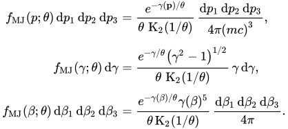
Note that when the MB distribution clearly deviates from the MJ distribution of the same temperature and dimensionality, one can misinterpret and deduce a different MB distribution that will give a good approximation to the MJ distribution. This new MB distribution can be either:
- a convected MB distribution, that is, an MB distribution with the same dimensionality, but with different temperature
 and bulk speed (or bulk energy
 )
- an MB distribution with the same bulk speed, but with different temperature and degrees of freedom
 . These two types of approximations are illustrated.
Other properties
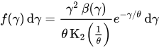
The MJ probability density function is given by:
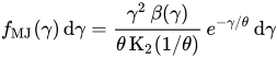
This means that a relativistic non-quantum particle with parameter has a probability of  of having its Lorentz factor in the interval
 .
Cumulative distribution function
The MJ cumulative distribution function is given by:

That has a series expansion at  :

By definition  , regardless of the parameter .
Average speed
To find the average speed,  , one must compute
 , where
 is the speed in terms of its Lorentz factor.
The integral simplifies to the closed-form expression:
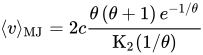
This closed formula for has a series expansion at  :

Or substituting the definition for the parameter :

Where the first term of the expansion, which is independently of  , corresponds to the average speed in the Maxwell–Boltzmann distribution,
 , whilst the following are relativistic corrections.
This closed formula for has a series expansion at  :

Or substituting the definition for the parameter :

Where it follows that is an upper limit to the particle's speed, something only present in a relativistic context, and not in the Maxwell–Boltzmann distribution.











 This article incorporates text by George Livadiotis available under the CC BY 3.0 license.

