Definition
The Rogers–Ramanujan identities are
G
(
q
)
=
∑
n
=
0
∞
q
n
2
(
q
;
q
)
n
=
1
(
q
;
q
5
)
∞
(
q
4
;
q
5
)
∞
=
1
+
q
+
q
2
+
q
3
+
2
q
4
+
2
q
5
+
3
q
6
+
⋯
{\displaystyle G(q)=\sum _{n=0}^{\infty }{\frac {q^{n^{2}}}{(q;q)_{n}}}={\frac {1}{(q;q^{5})_{\infty }(q^{4};q^{5})_{\infty }}}=1+q+q^{2}+q^{3}+2q^{4}+2q^{5}+3q^{6}+\cdots }
(sequence A003114 in the OEIS ) and
H
(
q
)
=
∑
n
=
0
∞
q
n
2
+
n
(
q
;
q
)
n
=
1
(
q
2
;
q
5
)
∞
(
q
3
;
q
5
)
∞
=
1
+
q
2
+
q
3
+
q
4
+
q
5
+
2
q
6
+
⋯
{\displaystyle H(q)=\sum _{n=0}^{\infty }{\frac {q^{n^{2}+n}}{(q;q)_{n}}}={\frac {1}{(q^{2};q^{5})_{\infty }(q^{3};q^{5})_{\infty }}}=1+q^{2}+q^{3}+q^{4}+q^{5}+2q^{6}+\cdots }
(sequence A003106 in the OEIS ) .Here,
(
a
;
q
)
n
{\displaystyle (a;q)_{n}}
q-Pochhammer symbol .
Application to partitions
Since the terms occurring in the identity are generating functions of certain partitions , the identities make statements about partitions (decompositions) of natural numbers . The number sequences resulting from the coefficients of the Maclaurin series of the Rogers–Ramanujan functions G and H are special partition number sequences of level 5:
G
(
x
)
=
1
(
x
;
x
5
)
∞
(
x
4
;
x
5
)
∞
=
1
+
∑
n
=
1
∞
P
G
(
n
)
x
n
{\displaystyle G(x)={\frac {1}{(x;x^{5})_{\infty }(x^{4};x^{5})_{\infty }}}=1+\sum _{n=1}^{\infty }P_{G}(n)x^{n}}
H
(
x
)
=
1
(
x
2
;
x
5
)
∞
(
x
3
;
x
5
)
∞
=
1
+
∑
n
=
1
∞
P
H
(
n
)
x
n
{\displaystyle H(x)={\frac {1}{(x^{2};x^{5})_{\infty }(x^{3};x^{5})_{\infty }}}=1+\sum _{n=1}^{\infty }P_{H}(n)x^{n}}
The number sequence
P
G
(
n
)
{\displaystyle P_{G}(n)}
(sequence A003114 in the OEIS ) [ 1]
N
0
{\displaystyle \mathbb {N} _{0}}
P
G
(
n
)
{\displaystyle P_{G}(n)}
And the number sequence
P
H
(
n
)
{\displaystyle P_{H}(n)}
(sequence A003106 in the OEIS ) [ 2]
N
0
{\displaystyle \mathbb {N} _{0}}
P
H
(
n
)
{\displaystyle P_{H}(n)}
Partition number sequence
P
G
(
n
)
{\displaystyle P_{G}(n)}
Natural number n
P
G
(
n
)
{\displaystyle P_{G}(n)}
Sum representations with the described criteria
1
1
1
2
1
1+1
3
1
1+1+1
4
2
4, 1+1+1+1
5
2
4+1, 1+1+1+1+1
6
3
6, 4+1+1, 1+1+1+1+1+1
7
3
6+1, 4+1+1+1, 1+1+1+1+1+1+1
8
4
6+1+1, 4+4, 4+1+1+1+1, 1+1+1+1+1+1+1+1
9
5
9, 6+1+1+1, 4+4+1, 4+1+1+1+1+1, 1+1+1+1+1+1+1+1+1
10
6
9+1, 6+4, 6+1+1+1+1, 4+4+1+1, 4+1+1+1+1+1+1, 1+1+1+1+1+1+1+1+1+1
11
7
11, 9+1+1, 6+4+1, 6+1+1+1+1+1, 4+4+1+1+1, 4+1+1+1+1+1+1+1, 1+1+1+1+1+1+1+1+1+1+1
12
9
11+1, 9+1+1+1, 6+6, 6+4+1+1, 6+1+1+1+1+1+1, 4+4+4, 4+4+1+1+1+1, 4+1+1+1+1+1+1+1+1, 1+1+1+1+1+1+1+1+1+1+1+1
13
10
11+1+1, 9+4, 9+1+1+1+1, 6+6+1, 6+4+1+1+1, 6+1+1+1+1+1+1+1, 4+4+4+1, 4+4+1+1+1+1+1, 4+1+1+1+1+1+1+1+1+1, 1+1+1+1+1+1+1+1+1+1+1+1+1
14
12
14, 11+1+1+1, 9+4+1, 9+1+1+1+1+1, 6+6+1+1, 6+4+4, 6+4+1+1+1+1, 6+1+1+1+1+1+1+1+1, 4+4+4+1+1, 4+4+1+1+1+1+1+1, 4+1+1+1+1+1+1+1+1+1+1, 1+1+1+1+1+1+1+1+1+1+1+1+1+1
15
14
14+1, 11+4, 11+1+1+1+1, 9+6, 9+4+1+1, 9+1+1+1+1+1+1, 6+6+1+1+1, 6+4+4+1, 6+4+1+1+1+1+1, 6+1+1+1+1+1+1+1+1+1, 4+4+4+1+1+1, 4+4+1+1+1+1+1+1+1, 4+1+1+1+1+1+1+1+1+1+1+1, 1+1+1+1+1+1+1+1+1+1+1+1+1+1+1
16
17
16, 14+1+1, 11+4+1, 11+1+1+1+1+1, 9+6+1, 9+4+1+1+1, 9+1+1+1+1+1+1+1, 6+6+4, 6+6+1+1+1+1, 6+4+4+1+1, 6+4+1+1+1+1+1+1, 6+1+1+1+1+1+1+1+1+1+1, 4+4+4+4, 4+4+4+1+1+1+1, 4+4+1+1+1+1+1+1+1+1, 4+1+1+1+1+1+1+1+1+1+1+1+1, 1+1+1+1+1+1+1+1+1+1+1+1+1+1+1+1
Partition number sequence
P
H
(
n
)
{\displaystyle P_{H}(n)}
Natural number n
P
H
(
n
)
{\displaystyle P_{H}(n)}
Sum representations with the described criteria
1
0
none
2
1
2
3
1
3
4
1
2+2
5
1
3+2
6
2
3+3, 2+2+2
7
2
7, 3+2+2
8
3
8, 3+3+2, 2+2+2+2
9
3
7+2, 3+3+3, 3+2+2+2
10
4
8+2, 7+3, 3+3+2+2, 2+2+2+2+2
Definition of the continued fractions
Domain coloring representation of the convergent
A
400
(
q
)
/
B
400
(
q
)
{\displaystyle A_{400}(q)/B_{400}(q)}
q
−
1
/
5
R
(
q
)
{\displaystyle q^{-1/5}R(q)}
R
(
q
)
{\displaystyle R(q)}
Representation of the approximation
q
1
/
5
A
400
(
q
)
/
B
400
(
q
)
{\displaystyle q^{1/5}A_{400}(q)/B_{400}(q)}
The following continued fraction
R
(
q
)
{\displaystyle R(q)}
Rogers–Ramanujan continued fraction ,[ 3] [ 4]
S
(
q
)
{\displaystyle S(q)}
Standardized continued fraction
Alternating continued fraction
R
(
q
)
=
q
1
/
5
[
1
+
q
1
+
q
2
1
+
q
3
1
+
⋯
]
{\displaystyle R(q)=q^{1/5}\left[1+{\frac {q}{1+{\frac {q^{2}}{1+{\frac {q^{3}}{1+\cdots }}}}}}\right]}
S
(
q
)
=
q
1
/
5
[
1
−
q
1
+
q
2
1
−
q
3
1
+
⋯
]
{\displaystyle S(q)=q^{1/5}\left[1-{\frac {q}{1+{\frac {q^{2}}{1-{\frac {q^{3}}{1+\cdots }}}}}}\right]}
The factor
q
1
5
{\displaystyle q^{\frac {1}{5}}}
This definition applies[ 5]
R
(
q
)
=
q
1
/
5
(
q
;
q
5
)
∞
(
q
4
;
q
5
)
∞
(
q
2
;
q
5
)
∞
(
q
3
;
q
5
)
∞
{\displaystyle R(q)=q^{1/5}{\frac {(q;q^{5})_{\infty }(q^{4};q^{5})_{\infty }}{(q^{2};q^{5})_{\infty }(q^{3};q^{5})_{\infty }}}}
R
(
q
)
=
q
1
/
5
∏
k
=
0
∞
(
1
−
q
5
k
+
1
)
(
1
−
q
5
k
+
4
)
(
1
−
q
5
k
+
2
)
(
1
−
q
5
k
+
3
)
=
q
1
/
5
H
(
q
)
G
(
q
)
{\displaystyle R(q)=q^{1/5}\prod _{k=0}^{\infty }{\frac {(1-q^{5k+1})(1-q^{5k+4})}{(1-q^{5k+2})(1-q^{5k+3})}}=q^{1/5}{\frac {H(q)}{G(q)}}}
This is the definition of the Ramanujan theta function :
f
(
a
,
b
)
=
∑
k
=
−
∞
∞
a
k
(
k
+
1
)
2
b
k
(
k
−
1
)
2
{\displaystyle f(a,b)=\sum _{k=-\infty }^{\infty }a^{\frac {k(k+1)}{2}}b^{\frac {k(k-1)}{2}}}
With this function, the continued fraction R can be created this way:
R
(
q
)
=
q
1
/
5
f
(
−
q
,
−
q
4
)
f
(
−
q
2
,
−
q
3
)
{\displaystyle R(q)=q^{1/5}{\frac {f(-q,-q^{4})}{f(-q^{2},-q^{3})}}}
The connection between the continued fraction and the Rogers–Ramanujan functions was already found by Rogers in 1894 (and later independently by Ramanujan).
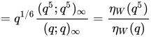
The continued fraction can also be expressed by the Dedekind eta function :[ 6]
R
(
q
)
=
tan
{
1
2
arccot
[
η
W
(
q
1
/
5
)
2
η
W
(
q
5
)
+
1
2
]
}
{\displaystyle R(q)=\tan {\biggl \{}{\frac {1}{2}}\operatorname {arccot} {\biggl [}{\frac {\eta _{W}(q^{1/5})}{2\eta _{W}(q^{5})}}+{\frac {1}{2}}{\biggr ]}{\biggr \}}}
The alternating continued fraction
S
(
q
)
{\displaystyle S(q)}
S
(
q
)
=
q
1
/
5
H
(
−
q
)
G
(
−
q
)
{\displaystyle S(q)=q^{1/5}{\frac {H(-q)}{G(-q)}}}
S
(
q
)
=
q
1
/
5
f
(
q
,
−
q
4
)
f
(
−
q
2
,
q
3
)
{\displaystyle S(q)=q^{1/5}{\frac {f(q,-q^{4})}{f(-q^{2},q^{3})}}}
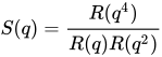
S
(
q
)
=
R
(
q
4
)
R
(
q
)
R
(
q
2
)
{\displaystyle S(q)={\frac {R(q^{4})}{R(q)R(q^{2})}}}
S
(
q
)
=
q
1
/
5
G
(
q
)
G
(
q
2
)
H
(
q
4
)
H
(
q
)
H
(
q
2
)
G
(
q
4
)
{\displaystyle S(q)=q^{1/5}{\frac {G(q)G(q^{2})H(q^{4})}{H(q)H(q^{2})G(q^{4})}}}
Modular modified functions of G and H
An elliptic function is a modular function if this function in dependence on the elliptic nome as an internal variable function results in a function, which also results as an algebraic combination of Legendre's elliptic modulus and its complete elliptic integrals of the first kind in the K and K' form. The Legendre's elliptic modulus is the numerical eccentricity of the corresponding ellipse.
If you set
q
=
e
2
π
i
τ
{\displaystyle q=e^{2\pi i\tau }}
τ
∈
C
{\displaystyle \tau \in \mathbb {C} }
modular functions !
G
M
(
q
)
=
q
−
1
60
G
(
q
)
{\displaystyle G_{M}(q)=q^{\frac {-1}{60}}G(q)}
H
M
(
q
)
=
q
11
60
H
(
q
)
{\displaystyle H_{M}(q)=q^{\frac {11}{60}}H(q)}
If q = e2πiτ , then q − 1/60G (q ) and q 11/60 H (q ) are modular functions of τ.
For the Rogers–Ramanujan continued fraction R(q) this formula is valid based on the described modular modifications of G and H:
R
(
q
)
=
H
M
(
q
)
G
M
(
q
)
{\displaystyle R(q)={\frac {H_{M}(q)}{G_{M}(q)}}}
Special values
These functions have the following values for the reciprocal of Gelfond's constant and for the square of this reciprocal:
G
M
[
exp
(
−
π
)
]
=
2
−
1
/
2
5
−
1
/
4
(
5
−
1
)
1
/
4
(
5
4
+
1
)
1
/
2
R
[
exp
(
−
π
)
]
−
1
/
2
=
=
2
1
/
4
5
−
1
/
8
Φ
1
/
2
cos
[
1
4
arctan
(
2
)
+
1
2
arcsin
(
Φ
−
2
)
]
{\displaystyle {\begin{aligned}G_{M}{\bigl [}\exp(-\pi ){\bigr ]}&=2^{-1/2}5^{-1/4}({\sqrt {5}}-1)^{1/4}({\sqrt[{4}]{5}}+1)^{1/2}R{\bigl [}\exp(-\pi ){\bigr ]}^{-1/2}=\\[4pt]&=2^{1/4}\,5^{-1/8}\,\Phi ^{1/2}\,{\color {blue}\cos {\bigl [}{\tfrac {1}{4}}\arctan(2)+{\tfrac {1}{2}}\arcsin(\Phi ^{-2}){\bigr ]}}\end{aligned}}}
H
M
[
exp
(
−
π
)
]
=
2
−
1
/
2
5
−
1
/
4
(
5
−
1
)
1
/
4
(
5
4
+
1
)
1
/
2
R
[
exp
(
−
π
)
]
1
/
2
=
=
2
1
/
4
5
−
1
/
8
Φ
1
/
2
sin
[
1
4
arctan
(
2
)
+
1
2
arcsin
(
Φ
−
2
)
]
{\displaystyle {\begin{aligned}H_{M}{\bigl [}\exp(-\pi ){\bigr ]}&=2^{-1/2}5^{-1/4}({\sqrt {5}}-1)^{1/4}({\sqrt[{4}]{5}}+1)^{1/2}R{\bigl [}\exp(-\pi ){\bigr ]}^{1/2}=\\[4pt]&=2^{1/4}\,5^{-1/8}\,\Phi ^{1/2}\,{\color {blue}\sin {\bigl [}{\tfrac {1}{4}}\arctan(2)+{\tfrac {1}{2}}\arcsin(\Phi ^{-2}){\bigr ]}}\end{aligned}}}
G
M
[
exp
(
−
2
π
)
]
=
10
−
1
/
4
(
5
−
1
)
1
/
4
R
[
exp
(
−
2
π
)
]
−
1
/
2
=
=
2
1
/
2
5
−
1
/
8
cos
[
1
4
arctan
(
2
)
]
{\displaystyle {\begin{aligned}G_{M}{\bigl [}\exp(-2\pi ){\bigr ]}&=10^{-1/4}({\sqrt {5}}-1)^{1/4}R{\bigl [}\exp(-2\pi ){\bigr ]}^{-1/2}=\\[4pt]&=2^{1/2}\,5^{-1/8}\,{\color {blue}\cos {\bigl [}{\tfrac {1}{4}}\arctan(2){\bigr ]}}\end{aligned}}}
H
M
[
exp
(
−
2
π
)
]
=
10
−
1
/
4
(
5
−
1
)
1
/
4
R
[
exp
(
−
2
π
)
]
1
/
2
=
=
2
1
/
2
5
−
1
/
8
sin
[
1
4
arctan
(
2
)
]
{\displaystyle {\begin{aligned}H_{M}{\bigl [}\exp(-2\pi ){\bigr ]}&=10^{-1/4}({\sqrt {5}}-1)^{1/4}R{\bigl [}\exp(-2\pi ){\bigr ]}^{1/2}=\\[4pt]&=2^{1/2}\,5^{-1/8}\,{\color {blue}\sin {\bigl [}{\tfrac {1}{4}}\arctan(2){\bigr ]}}\end{aligned}}}
The Rogers–Ramanujan continued fraction takes the following ordinate values for these abscissa values:
R
[
exp
(
−
π
)
]
=
1
4
(
5
+
1
)
(
5
−
5
+
2
)
(
5
+
2
+
5
4
)
=
=
Φ
3
/
2
cl
(
1
5
ϖ
)
−
3
/
2
cl
(
2
5
ϖ
)
3
/
2
cl
(
1
10
ϖ
)
2
cl
(
3
10
ϖ
)
slh
(
2
5
2
ϖ
)
=
=
tan
[
1
4
arctan
(
2
)
+
1
2
arcsin
(
Φ
−
2
)
]
{\displaystyle {\begin{aligned}R[\exp(-\pi )]{}&={\tfrac {1}{4}}({\sqrt {5}}+1)({\sqrt {5}}-{\sqrt {{\sqrt {5}}+2}})({\sqrt {{\sqrt {5}}+2}}+{\sqrt[{4}]{5}})=\\[4pt]&{}=\Phi ^{3/2}\operatorname {cl} ({\tfrac {1}{5}}\varpi )^{-3/2}\operatorname {cl} ({\tfrac {2}{5}}\varpi )^{3/2}\operatorname {cl} ({\tfrac {1}{10}}\varpi )^{2}\operatorname {cl} ({\tfrac {3}{10}}\varpi )\operatorname {slh} ({\tfrac {2}{5}}{\sqrt {2}}\,\varpi )=\\[4pt]&{}={\color {blue}\tan {\bigl [}{\tfrac {1}{4}}\arctan(2)+{\tfrac {1}{2}}\arcsin(\Phi ^{-2}){\bigr ]}}\\[4pt]\end{aligned}}}
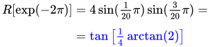
R
[
exp
(
−
2
π
)
]
=
4
sin
(
1
20
π
)
sin
(
3
20
π
)
=
=
tan
[
1
4
arctan
(
2
)
]
{\displaystyle {\begin{aligned}R[\exp(-2\pi )]{}&=4\sin({\tfrac {1}{20}}\pi )\sin({\tfrac {3}{20}}\pi )=\\[4pt]&{}={\color {blue}\tan {\bigl [}{\tfrac {1}{4}}\arctan(2){\bigr ]}}\end{aligned}}}
Dedekind eta function identities
Pentagonal number theorem
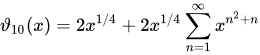
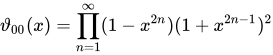
For the Dedekind eta function according to Weber's definition[ 10]
η
W
(
x
)
=
2
−
1
/
6
ϑ
10
(
x
)
1
/
6
ϑ
00
(
x
)
1
/
6
ϑ
01
(
x
)
2
/
3
{\displaystyle \eta _{W}(x)=2^{-1/6}\vartheta _{10}(x)^{1/6}\vartheta _{00}(x)^{1/6}\vartheta _{01}(x)^{2/3}}
η
W
(
x
)
=
2
−
1
/
3
ϑ
10
(
x
1
/
2
)
1
/
3
ϑ
00
(
x
1
/
2
)
1
/
3
ϑ
01
(
x
1
/
2
)
1
/
3
{\displaystyle \eta _{W}(x)=2^{-1/3}\vartheta _{10}(x^{1/2})^{1/3}\vartheta _{00}(x^{1/2})^{1/3}\vartheta _{01}(x^{1/2})^{1/3}}
η
W
(
x
)
=
x
1
/
24
∏
n
=
1
∞
(
1
−
x
n
)
=
x
1
/
24
(
x
;
x
)
∞
{\displaystyle \eta _{W}(x)=x^{1/24}\prod _{n=1}^{\infty }(1-x^{n})=x^{1/24}(x;x)_{\infty }}
η
W
(
x
)
=
x
1
/
24
{
1
+
∑
n
=
1
∞
[
−
x
Fn
(
2
n
−
1
)
−
x
Kr
(
2
n
−
1
)
+
x
Fn
(
2
n
)
+
x
Kr
(
2
n
)
]
}
{\displaystyle \eta _{W}(x)=x^{1/24}{\biggl \{}1+\sum _{n=1}^{\infty }{\bigl [}-x^{{\text{Fn}}(2n-1)}-x^{{\text{Kr}}(2n-1)}+x^{{\text{Fn}}(2n)}+x^{{\text{Kr}}(2n)}{\bigr ]}{\biggr \}}}
η
W
(
x
)
=
x
1
/
24
{
1
+
∑
n
=
1
∞
P
(
n
)
x
n
}
−
1
{\displaystyle \eta _{W}(x)=x^{1/24}{\biggl \{}1+\sum _{n=1}^{\infty }\mathrm {P} (n)\,x^{n}{\biggr \}}^{-1}}
The fourth formula describes the pentagonal number theorem [ 11]
These basic definitions apply to the pentagonal numbers and the card house numbers :
Fn
(
z
)
=
1
2
z
(
3
z
−
1
)
{\displaystyle {\text{Fn}}(z)={\tfrac {1}{2}}z(3z-1)}
Kr
(
z
)
=
1
2
z
(
3
z
+
1
)
{\displaystyle {\text{Kr}}(z)={\tfrac {1}{2}}z(3z+1)}
The fifth formula contains the Regular Partition Numbers as coefficients.
The Regular Partition Number Sequence
P
(
n
)
{\displaystyle \mathrm {P} (n)}
integer number
n
{\displaystyle n}
n
=
1
{\displaystyle n=1}
n
=
5
{\displaystyle n=5}
P
{\displaystyle P}
Example values of P(n) and associated number partitions
n
P(n)
Corresponding partitions
1
1
(1)
2
2
(1+1), (2)
3
3
(1+1+1), (1+2), (3)
4
5
(1+1+1+1), (1+1+2), (2+2), (1+3), (4)
5
7
(1+1+1+1+1), (1+1+1+2), (1+2+2), (1+1+3), (2+3), (1+4), (5)
6
11
(1+1+1+1+1+1), (1+1+1+1+2), (1+1+2+2), (2+2+2), (1+1+1+3), (1+2+3), (3+3), (1+1+4), (2+4), (1+5), (6)
Reduced Weber modular function
The Weber modular functions in their reduced form are an efficient way of computing the values of the Rogers–Ramanujan functions:
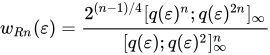
First of all we introduce the reduced Weber modular functions in that pattern:
w
R
n
(
ε
)
=
2
(
n
−
1
)
/
4
[
q
(
ε
)
n
;
q
(
ε
)
2
n
]
∞
[
q
(
ε
)
;
q
(
ε
)
2
]
∞
n
{\displaystyle w_{Rn}(\varepsilon )={\frac {2^{(n-1)/4}[q(\varepsilon )^{n};q(\varepsilon )^{2n}]_{\infty }}{[q(\varepsilon );q(\varepsilon )^{2}]_{\infty }^{n}}}}
w
R
5
(
ε
)
=
2
[
q
(
ε
)
5
;
q
(
ε
)
10
]
∞
[
q
(
ε
)
;
q
(
ε
)
2
]
∞
5
{\displaystyle w_{R5}(\varepsilon )={\frac {2[q(\varepsilon )^{5};q(\varepsilon )^{10}]_{\infty }}{[q(\varepsilon );q(\varepsilon )^{2}]_{\infty }^{5}}}}
This function fulfills following equation of sixth degree:
w
R
5
(
ε
)
6
−
2
w
R
5
(
ε
)
5
=
tan
[
2
arctan
(
ε
)
]
2
[
2
w
R
5
(
ε
)
+
1
]
{\displaystyle w_{R5}(\varepsilon )^{6}-2\,w_{R5}(\varepsilon )^{5}=\tan {\bigl [}2\arctan(\varepsilon ){\bigr ]}^{2}{\bigl [}2\,w_{R5}(\varepsilon )+1{\bigr ]}}
Therefore this
w
R
5
{\displaystyle w_{R5}}
algebraic function indeed.
But along with the Abel–Ruffini theorem this function in relation to the eccentricity can not be represented by elementary expressions.
However there are many values that in fact can be expressed elementarily.
Four examples shall be given for this:
First example:
w
R
5
(
1
2
2
)
6
−
2
w
R
5
(
1
2
2
)
5
=
16
w
R
5
(
1
2
2
)
+
8
{\displaystyle w_{R5}({\tfrac {1}{2}}{\sqrt {2}})^{6}-2\,w_{R5}({\tfrac {1}{2}}{\sqrt {2}})^{5}=16\,w_{R5}({\tfrac {1}{2}}{\sqrt {2}})+8}
w
R
5
(
1
2
2
)
=
5
4
+
1
{\displaystyle w_{R5}({\tfrac {1}{2}}{\sqrt {2}})={\sqrt[{4}]{5}}+1}
Second example:
Third example:
w
R
5
[
(
2
−
3
)
(
3
−
2
)
]
6
−
2
w
R
5
[
(
2
−
3
)
(
3
−
2
)
]
5
=
(
2
−
1
)
4
{
2
w
R
5
[
(
2
−
3
)
(
3
−
2
)
]
+
1
}
{\displaystyle w_{R5}{\bigl [}(2-{\sqrt {3}})({\sqrt {3}}-{\sqrt {2}}){\bigr ]}^{6}-2\,w_{R5}{\bigl [}(2-{\sqrt {3}})({\sqrt {3}}-{\sqrt {2}}){\bigr ]}^{5}=({\sqrt {2}}-1)^{4}{\bigl \{}2\,w_{R5}[(2-{\sqrt {3}})({\sqrt {3}}-{\sqrt {2}}){\bigr ]}+1{\bigr \}}}
w
R
5
[
(
2
−
3
)
(
3
−
2
)
]
=
cot
[
1
4
π
−
1
4
arccsc
(
1
4
10
+
1
4
)
]
{\displaystyle w_{R5}[(2-{\sqrt {3}})({\sqrt {3}}-{\sqrt {2}}){\bigr ]}=\cot {\bigl [}{\tfrac {1}{4}}\pi -{\tfrac {1}{4}}\operatorname {arccsc}({\tfrac {1}{4}}{\sqrt {10}}+{\tfrac {1}{4}}){\bigr ]}}
Fourth example:
w
R
5
[
(
2
−
3
)
(
3
+
2
)
]
6
−
2
w
R
5
[
(
2
−
3
)
(
3
+
2
)
]
5
=
(
2
+
1
)
4
{
2
w
R
5
[
(
2
−
3
)
(
3
+
2
)
]
+
1
}
{\displaystyle w_{R5}{\bigl [}(2-{\sqrt {3}})({\sqrt {3}}+{\sqrt {2}}){\bigr ]}^{6}-2\,w_{R5}{\bigl [}(2-{\sqrt {3}})({\sqrt {3}}+{\sqrt {2}}){\bigr ]}^{5}=({\sqrt {2}}+1)^{4}{\bigl \{}2\,w_{R5}[(2-{\sqrt {3}})({\sqrt {3}}+{\sqrt {2}}){\bigr ]}+1{\bigr \}}}
w
R
5
[
(
2
−
3
)
(
3
+
2
)
]
=
cot
[
1
4
arccsc
(
1
4
10
+
1
4
)
]
{\displaystyle w_{R5}[(2-{\sqrt {3}})({\sqrt {3}}+{\sqrt {2}}){\bigr ]}=\cot {\bigl [}{\tfrac {1}{4}}\operatorname {arccsc}({\tfrac {1}{4}}{\sqrt {10}}+{\tfrac {1}{4}}){\bigr ]}}
For that function, a further expression is valid:
w
R
5
(
ε
)
=
5
ϑ
01
[
q
(
k
)
5
]
2
2
ϑ
01
[
q
(
k
)
]
2
−
1
2
{\displaystyle w_{R5}(\varepsilon )={\frac {5\,\vartheta _{01}[q(k)^{5}]^{2}}{2\,\vartheta _{01}[q(k)]^{2}}}-{\frac {1}{2}}}
Exact eccentricity identity for the functions G and H
In this way the accurate eccentricity dependent formulas for the functions G and H can be generated:
Following Dedekind eta function quotient has this eccentricity dependency:
η
W
[
q
(
ε
)
2
]
η
W
[
q
(
ε
)
]
=
2
−
1
/
4
tan
[
2
arctan
(
ε
)
]
1
/
12
{\displaystyle {\frac {\eta _{W}[q(\varepsilon )^{2}]}{\eta _{W}[q(\varepsilon )]}}=2^{-1/4}\tan {\bigl [}2\arctan(\varepsilon ){\bigr ]}^{1/12}}
This is the eccentricity dependent formula for the continued fraction R:
R
[
q
(
ε
)
]
=
tan
{
1
2
arctan
[
w
R
5
(
ε
)
−
2
2
w
R
5
(
ε
)
+
1
]
}
1
/
5
tan
{
1
2
arccot
[
w
R
5
(
ε
)
−
2
2
w
R
5
(
ε
)
+
1
]
}
2
/
5
{\displaystyle R[q(\varepsilon )]=\tan {\biggl \{}{\frac {1}{2}}\arctan {\biggl [}{\frac {w_{R5}(\varepsilon )-2}{2\,w_{R5}(\varepsilon )+1}}{\biggr ]}{\biggr \}}^{1/5}\tan {\biggl \{}{\frac {1}{2}}\operatorname {arccot} {\biggl [}{\frac {w_{R5}(\varepsilon )-2}{2\,w_{R5}(\varepsilon )+1}}{\biggr ]}{\biggr \}}^{2/5}}
The last three now mentioned formulas will be inserted into the final formulas mentioned in the section above:
G
M
[
q
(
ε
)
]
=
tan
[
2
arctan
(
ε
)
]
1
/
6
[
2
w
R
5
(
ε
)
+
1
]
1
/
4
5
1
/
4
w
R
5
(
ε
)
1
/
2
tan
{
1
2
arctan
[
w
R
5
(
ε
)
−
2
2
w
R
5
(
ε
)
+
1
]
}
−
1
/
10
tan
{
1
2
arccot
[
w
R
5
(
ε
)
−
2
2
w
R
5
(
ε
)
+
1
]
}
−
1
/
5
{\displaystyle G_{M}{\bigl [}q(\varepsilon ){\bigr ]}={\frac {\tan {\bigl [}2\arctan(\varepsilon ){\bigr ]}^{1/6}{\bigl [}2\,w_{R5}(\varepsilon )+1{\bigr ]}^{1/4}}{5^{1/4}w_{R5}(\varepsilon )^{1/2}}}\tan {\biggl \{}{\frac {1}{2}}\arctan {\biggl [}{\frac {w_{R5}(\varepsilon )-2}{2\,w_{R5}(\varepsilon )+1}}{\biggr ]}{\biggr \}}^{-1/10}\tan {\biggl \{}{\frac {1}{2}}\operatorname {arccot} {\biggl [}{\frac {w_{R5}(\varepsilon )-2}{2\,w_{R5}(\varepsilon )+1}}{\biggr ]}{\biggr \}}^{-1/5}}
H
M
[
q
(
ε
)
]
=
tan
[
2
arctan
(
ε
)
]
1
/
6
[
2
w
R
5
(
ε
)
+
1
]
1
/
4
5
1
/
4
w
R
5
(
ε
)
1
/
2
tan
{
1
2
arctan
[
w
R
5
(
ε
)
−
2
2
w
R
5
(
ε
)
+
1
]
}
1
/
10
tan
{
1
2
arccot
[
w
R
5
(
ε
)
−
2
2
w
R
5
(
ε
)
+
1
]
}
1
/
5
{\displaystyle H_{M}{\bigl [}q(\varepsilon ){\bigr ]}={\frac {\tan {\bigl [}2\arctan(\varepsilon ){\bigr ]}^{1/6}{\bigl [}2\,w_{R5}(\varepsilon )+1{\bigr ]}^{1/4}}{5^{1/4}w_{R5}(\varepsilon )^{1/2}}}\tan {\biggl \{}{\frac {1}{2}}\arctan {\biggl [}{\frac {w_{R5}(\varepsilon )-2}{2\,w_{R5}(\varepsilon )+1}}{\biggr ]}{\biggr \}}^{1/10}\tan {\biggl \{}{\frac {1}{2}}\operatorname {arccot} {\biggl [}{\frac {w_{R5}(\varepsilon )-2}{2\,w_{R5}(\varepsilon )+1}}{\biggr ]}{\biggr \}}^{1/5}}
On the left side of the balances the functions
G
M
(
q
)
{\displaystyle G_{M}(q)}
H
M
(
q
)
{\displaystyle H_{M}(q)}
elliptic nome function
q
(
ε
)
{\displaystyle q(\varepsilon )}
And on the right side an algebraic combination of the eccentricity
ε
{\displaystyle \varepsilon }
Therefore these functions
G
M
(
q
)
=
q
−
1
/
60
G
(
q
)
{\displaystyle G_{M}(q)=q^{-1/60}G(q)}
H
M
(
q
)
=
q
11
/
60
H
(
q
)
{\displaystyle H_{M}(q)=q^{11/60}H(q)}
Application to quintic equations
Discovery of the corresponding modulus by Charles Hermite
The general case of quintic equations in the Bring–Jerrard form has a non-elementary solution based on the Abel–Ruffini theorem and will now be explained using the elliptic nome of the corresponding modulus, described by the lemniscate elliptic functions in a simplified way.
x
5
+
5
x
=
4
c
{\displaystyle x^{5}+5\,x=4\,c}
The real solution for all real values
c
∈
R
{\displaystyle c\in \mathbb {R} }
x
=
S
⟨
q
{
ctlh
[
1
2
aclh
(
c
)
]
2
}
⟩
2
−
R
⟨
q
{
ctlh
[
1
2
aclh
(
c
)
]
2
}
2
⟩
S
⟨
q
{
ctlh
[
1
2
aclh
(
c
)
]
2
}
⟩
2
×
×
1
−
R
⟨
q
{
ctlh
[
1
2
aclh
(
c
)
]
2
}
2
⟩
S
⟨
q
{
ctlh
[
1
2
aclh
(
c
)
]
2
}
⟩
R
⟨
q
{
ctlh
[
1
2
aclh
(
c
)
]
2
}
2
⟩
2
×
×
ϑ
00
⟨
q
{
ctlh
[
1
2
aclh
(
c
)
]
2
}
5
⟩
ϑ
00
⟨
q
{
ctlh
[
1
2
aclh
(
c
)
]
2
}
1
/
5
⟩
2
−
5
ϑ
00
⟨
q
{
ctlh
[
1
2
aclh
(
c
)
]
2
}
5
⟩
3
4
ϑ
10
⟨
q
{
ctlh
[
1
2
aclh
(
c
)
]
2
}
⟩
ϑ
01
⟨
q
{
ctlh
[
1
2
aclh
(
c
)
]
2
}
⟩
ϑ
00
⟨
q
{
ctlh
[
1
2
aclh
(
c
)
]
2
}
⟩
{\displaystyle {\begin{aligned}x={}&{\frac {S{\bigl \langle }q\{\operatorname {ctlh} [{\tfrac {1}{2}}\operatorname {aclh} (c)]^{2}\}{\bigr \rangle }^{2}-R{\bigl \langle }q\{\operatorname {ctlh} [{\tfrac {1}{2}}\operatorname {aclh} (c)]^{2}\}^{2}{\bigr \rangle }}{S{\bigl \langle }q\{\operatorname {ctlh} [{\tfrac {1}{2}}\operatorname {aclh} (c)]^{2}\}{\bigr \rangle }^{2}}}\times \\[4pt]&{}\times {\frac {1-R{\bigl \langle }q\{\operatorname {ctlh} [{\tfrac {1}{2}}\operatorname {aclh} (c)]^{2}\}^{2}{\bigr \rangle }\,S{\bigl \langle }q\{\operatorname {ctlh} [{\tfrac {1}{2}}\operatorname {aclh} (c)]^{2}\}{\bigr \rangle }}{R{\bigl \langle }q\{\operatorname {ctlh} [{\tfrac {1}{2}}\operatorname {aclh} (c)]^{2}\}^{2}{\bigr \rangle }^{2}}}\times \\[4pt]&{}\times {\frac {\vartheta _{00}{\bigl \langle }q\{\operatorname {ctlh} [{\tfrac {1}{2}}\operatorname {aclh} (c)]^{2}\}^{5}{\bigr \rangle }\,\vartheta _{00}{\bigl \langle }q\{\operatorname {ctlh} [{\tfrac {1}{2}}\operatorname {aclh} (c)]^{2}\}^{1/5}{\bigr \rangle }^{2}-5\,\vartheta _{00}{\bigl \langle }q\{\operatorname {ctlh} [{\tfrac {1}{2}}\operatorname {aclh} (c)]^{2}\}^{5}{\bigr \rangle }^{3}}{4\,\vartheta _{10}{\bigl \langle }q\{\operatorname {ctlh} [{\tfrac {1}{2}}\operatorname {aclh} (c)]^{2}\}{\bigr \rangle }\,\vartheta _{01}{\bigl \langle }q\{\operatorname {ctlh} [{\tfrac {1}{2}}\operatorname {aclh} (c)]^{2}\}{\bigr \rangle }\,\vartheta _{00}{\bigl \langle }q\{\operatorname {ctlh} [{\tfrac {1}{2}}\operatorname {aclh} (c)]^{2}\}{\bigr \rangle }}}\end{aligned}}}
Alternatively, the same solution can be presented in this way:
x
=
5
ϑ
00
(
Q
5
)
3
−
ϑ
00
(
Q
5
)
ϑ
00
(
Q
)
2
4
ϑ
10
(
Q
)
ϑ
01
(
Q
)
ϑ
00
(
Q
)
×
S
(
Q
)
2
+
R
(
Q
2
)
S
(
Q
)
×
[
R
(
Q
2
)
S
(
Q
)
+
R
(
Q
2
)
+
S
(
Q
)
−
1
]
w
i
t
h
Q
=
q
{
c
t
l
h
[
1
2
aclh
(
c
)
]
2
}
{\displaystyle {\begin{aligned}x={}&{\frac {5\,\vartheta _{00}(Q^{5})^{3}-\vartheta _{00}(Q^{5})\,\vartheta _{00}(Q)^{2}}{4\,\vartheta _{10}(Q)\,\vartheta _{01}(Q)\,\vartheta _{00}(Q)}}\times {\frac {S(Q)^{2}+R(Q^{2})}{S(Q)}}\times {\bigl [}R(Q^{2})S(Q)+R(Q^{2})+S(Q)-1{\bigr ]}\\[4pt]&\mathrm {with} \,\,Q=q{\bigl \{}\mathrm {ctlh} {\bigl [}{\tfrac {1}{2}}\operatorname {aclh} (c){\bigr ]}^{2}{\bigr \}}\end{aligned}}}
The mathematician Charles Hermite determined the value of the elliptic modulus k in relation to the coefficient of the absolute term of the Bring–Jerrard form. In his essay "Sur la résolution de l'Équation du cinquiéme degré Comptes rendus" he described the calculation method for the elliptic modulus in terms of the absolute term. The Italian version of his essay "Sulla risoluzione delle equazioni del quinto grado" contains exactly on page 258 the upper Bring–Jerrard equation formula, which can be solved directly with the functions based on the corresponding elliptic modulus. This corresponding elliptic modulus can be worked out by using the square of the Hyperbolic lemniscate cotangent. For the derivation of this, please see the Wikipedia article lemniscate elliptic functions !
The elliptic nome of this corresponding modulus is represented here with the letter Q:
Q
=
q
{
c
t
l
h
[
1
2
aclh
(
c
)
]
2
}
=
{\displaystyle Q=q{\bigl \{}\mathrm {ctlh} {\bigl [}{\tfrac {1}{2}}\operatorname {aclh} (c){\bigr ]}^{2}{\bigr \}}=}
=
q
[
(
c
4
+
1
+
1
+
c
)
(
2
c
2
+
2
+
2
c
4
+
1
)
−
1
/
2
]
{\displaystyle =q{\bigl [}{\bigl (}{\sqrt {{\sqrt {c^{4}+1}}+1}}+c{\bigr )}{\bigl (}2c^{2}+2+2{\sqrt {c^{4}+1}}\,{\bigr )}^{-1/2}{\bigr ]}}
The abbreviation ctlh expresses the Hyperbolic Lemniscate Cotangent and the abbreviation aclh represents the Hyperbolic Lemniscate Areacosine !
Calculation examples
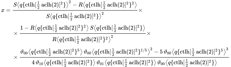
Two examples of this solution algorithm are now mentioned:
First calculation example:
Quintic Bring–Jerrard equation:
x
5
+
5
x
=
8
{\displaystyle x^{5}+5\,x=8}
Solution formula:
x
=
S
⟨
q
{
ctlh
[
1
2
aclh
(
2
)
]
2
}
⟩
2
−
R
⟨
q
{
ctlh
[
1
2
aclh
(
2
)
]
2
}
2
⟩
S
⟨
q
{
ctlh
[
1
2
aclh
(
2
)
]
2
}
⟩
2
×
×
1
−
R
⟨
q
{
ctlh
[
1
2
aclh
(
2
)
]
2
}
2
⟩
S
⟨
q
{
ctlh
[
1
2
aclh
(
2
)
]
2
}
⟩
R
⟨
q
{
ctlh
[
1
2
aclh
(
2
)
]
2
}
2
⟩
2
×
×
ϑ
00
⟨
q
{
ctlh
[
1
2
aclh
(
2
)
]
2
}
5
⟩
ϑ
00
⟨
q
{
ctlh
[
1
2
aclh
(
2
)
]
2
}
1
/
5
⟩
2
−
5
ϑ
00
⟨
q
{
ctlh
[
1
2
aclh
(
2
)
]
2
}
5
⟩
3
4
ϑ
10
⟨
q
{
ctlh
[
1
2
aclh
(
2
)
]
2
}
⟩
ϑ
01
⟨
q
{
ctlh
[
1
2
aclh
(
2
)
]
2
}
⟩
ϑ
00
⟨
q
{
ctlh
[
1
2
aclh
(
2
)
]
2
}
⟩
{\displaystyle {\begin{aligned}x={}&{\frac {S{\bigl \langle }q\{\operatorname {ctlh} [{\tfrac {1}{2}}\operatorname {aclh} (2)]^{2}\}{\bigr \rangle }^{2}-R{\bigl \langle }q\{\operatorname {ctlh} [{\tfrac {1}{2}}\operatorname {aclh} (2)]^{2}\}^{2}{\bigr \rangle }}{S{\bigl \langle }q\{\operatorname {ctlh} [{\tfrac {1}{2}}\operatorname {aclh} (2)]^{2}\}{\bigr \rangle }^{2}}}\times \\[4pt]&{}\times {\frac {1-R{\bigl \langle }q\{\operatorname {ctlh} [{\tfrac {1}{2}}\operatorname {aclh} (2)]^{2}\}^{2}{\bigr \rangle }\,S{\bigl \langle }q\{\operatorname {ctlh} [{\tfrac {1}{2}}\operatorname {aclh} (2)]^{2}\}{\bigr \rangle }}{R{\bigl \langle }q\{\operatorname {ctlh} [{\tfrac {1}{2}}\operatorname {aclh} (2)]^{2}\}^{2}{\bigr \rangle }^{2}}}\times \\[4pt]&{}\times {\frac {\vartheta _{00}{\bigl \langle }q\{\operatorname {ctlh} [{\tfrac {1}{2}}\operatorname {aclh} (2)]^{2}\}^{5}{\bigr \rangle }\,\vartheta _{00}{\bigl \langle }q\{\operatorname {ctlh} [{\tfrac {1}{2}}\operatorname {aclh} (2)]^{2}\}^{1/5}{\bigr \rangle }^{2}-5\,\vartheta _{00}{\bigl \langle }q\{\operatorname {ctlh} [{\tfrac {1}{2}}\operatorname {aclh} (2)]^{2}\}^{5}{\bigr \rangle }^{3}}{4\,\vartheta _{10}{\bigl \langle }q\{\operatorname {ctlh} [{\tfrac {1}{2}}\operatorname {aclh} (2)]^{2}\}{\bigr \rangle }\,\vartheta _{01}{\bigl \langle }q\{\operatorname {ctlh} [{\tfrac {1}{2}}\operatorname {aclh} (2)]^{2}\}{\bigr \rangle }\,\vartheta _{00}{\bigl \langle }q\{\operatorname {ctlh} [{\tfrac {1}{2}}\operatorname {aclh} (2)]^{2}\}{\bigr \rangle }}}\end{aligned}}}
Decimal places of the nome:
q
{
c
t
l
h
[
1
2
aclh
(
2
)
]
2
}
=
q
[
(
17
+
1
+
2
)
(
10
+
2
17
)
−
1
/
2
]
=
{\displaystyle q{\bigl \{}\mathrm {ctlh} {\bigl [}{\tfrac {1}{2}}\operatorname {aclh} (2){\bigr ]}^{2}{\bigr \}}=q{\bigl [}{\bigl (}{\sqrt {{\sqrt {17}}+1}}+2{\bigr )}{\bigl (}10+2{\sqrt {17}}{\bigr )}^{-1/2}{\bigr ]}=}
=
0,306
3466544466074265361088194021326272090461143559097382981847144
…
{\displaystyle =0{,}3063466544466074265361088194021326272090461143559097382981847144\ldots }
Decimal places of the solution:
x
=
1,167
0361837016430473110194319963961012975521104880199105205748723
…
{\displaystyle x=1{,}1670361837016430473110194319963961012975521104880199105205748723\ldots }
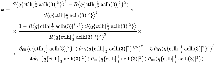
Second calculation example:
Quintic Bring–Jerrard equation:
x
5
+
5
x
=
12
{\displaystyle x^{5}+5\,x=12}
Solution:
x
=
S
⟨
q
{
ctlh
[
1
2
aclh
(
3
)
]
2
}
⟩
2
−
R
⟨
q
{
ctlh
[
1
2
aclh
(
3
)
]
2
}
2
⟩
S
⟨
q
{
ctlh
[
1
2
aclh
(
3
)
]
2
}
⟩
2
×
×
1
−
R
⟨
q
{
ctlh
[
1
2
aclh
(
3
)
]
2
}
2
⟩
S
⟨
q
{
ctlh
[
1
2
aclh
(
3
)
]
2
}
⟩
R
⟨
q
{
ctlh
[
1
2
aclh
(
3
)
]
2
}
2
⟩
2
×
×
ϑ
00
⟨
q
{
ctlh
[
1
2
aclh
(
3
)
]
2
}
5
⟩
ϑ
00
⟨
q
{
ctlh
[
1
2
aclh
(
3
)
]
2
}
1
/
5
⟩
2
−
5
ϑ
00
⟨
q
{
ctlh
[
1
2
aclh
(
3
)
]
2
}
5
⟩
3
4
ϑ
10
⟨
q
{
ctlh
[
1
2
aclh
(
3
)
]
2
}
⟩
ϑ
01
⟨
q
{
ctlh
[
1
2
aclh
(
3
)
]
2
}
⟩
ϑ
00
⟨
q
{
ctlh
[
1
2
aclh
(
3
)
]
2
}
⟩
{\displaystyle {\begin{aligned}x={}&{\frac {S{\bigl \langle }q\{\operatorname {ctlh} [{\tfrac {1}{2}}\operatorname {aclh} (3)]^{2}\}{\bigr \rangle }^{2}-R{\bigl \langle }q\{\operatorname {ctlh} [{\tfrac {1}{2}}\operatorname {aclh} (3)]^{2}\}^{2}{\bigr \rangle }}{S{\bigl \langle }q\{\operatorname {ctlh} [{\tfrac {1}{2}}\operatorname {aclh} (3)]^{2}\}{\bigr \rangle }^{2}}}\times \\[4pt]&{}\times {\frac {1-R{\bigl \langle }q\{\operatorname {ctlh} [{\tfrac {1}{2}}\operatorname {aclh} (3)]^{2}\}^{2}{\bigr \rangle }\,S{\bigl \langle }q\{\operatorname {ctlh} [{\tfrac {1}{2}}\operatorname {aclh} (3)]^{2}\}{\bigr \rangle }}{R{\bigl \langle }q\{\operatorname {ctlh} [{\tfrac {1}{2}}\operatorname {aclh} (3)]^{2}\}^{2}{\bigr \rangle }^{2}}}\times \\[4pt]&{}\times {\frac {\vartheta _{00}{\bigl \langle }q\{\operatorname {ctlh} [{\tfrac {1}{2}}\operatorname {aclh} (3)]^{2}\}^{5}{\bigr \rangle }\,\vartheta _{00}{\bigl \langle }q\{\operatorname {ctlh} [{\tfrac {1}{2}}\operatorname {aclh} (3)]^{2}\}^{1/5}{\bigr \rangle }^{2}-5\,\vartheta _{00}{\bigl \langle }q\{\operatorname {ctlh} [{\tfrac {1}{2}}\operatorname {aclh} (3)]^{2}\}^{5}{\bigr \rangle }^{3}}{4\,\vartheta _{10}{\bigl \langle }q\{\operatorname {ctlh} [{\tfrac {1}{2}}\operatorname {aclh} (3)]^{2}\}{\bigr \rangle }\,\vartheta _{01}{\bigl \langle }q\{\operatorname {ctlh} [{\tfrac {1}{2}}\operatorname {aclh} (3)]^{2}\}{\bigr \rangle }\,\vartheta _{00}{\bigl \langle }q\{\operatorname {ctlh} [{\tfrac {1}{2}}\operatorname {aclh} (3)]^{2}\}{\bigr \rangle }}}\end{aligned}}}
Decimal places of the nome:
q
{
c
t
l
h
[
1
2
aclh
(
3
)
]
2
}
=
q
[
(
82
+
1
+
3
)
(
20
+
2
82
)
−
1
/
2
]
=
{\displaystyle q{\bigl \{}\mathrm {ctlh} {\bigl [}{\tfrac {1}{2}}\operatorname {aclh} (3){\bigr ]}^{2}{\bigr \}}=q{\bigl [}{\bigl (}{\sqrt {{\sqrt {82}}+1}}+3{\bigr )}{\bigl (}20+2{\sqrt {82}}{\bigr )}^{-1/2}{\bigr ]}=}
=
0,370
6649511520240756244325221775686571518680899597473957509743879
…
{\displaystyle =0{,}3706649511520240756244325221775686571518680899597473957509743879\ldots }
Decimal places of the solution:
x
=
1,384
0917958231463592477551262671354748859350601806764501691889116
…
{\displaystyle x=1{,}3840917958231463592477551262671354748859350601806764501691889116\ldots }
Applications in Physics
The Rogers–Ramanujan identities appeared in Baxter's solution of the hard hexagon model in statistical mechanics .
The demodularized standard form of the Ramanujan's continued fraction unanchored from the modular form is as follows:
H
(
q
)
G
(
q
)
=
[
1
+
q
1
+
q
2
1
+
q
3
1
+
⋯
]
{\displaystyle {\frac {H(q)}{G(q)}}=\left[1+{\frac {q}{1+{\frac {q^{2}}{1+{\frac {q^{3}}{1+\cdots }}}}}}\right]}
Relations to affine Lie algebras and vertex operator algebras
James Lepowsky and Robert Lee Wilson were the first to prove Rogers–Ramanujan identities using completely representation-theoretic techniques. They proved these identities using level 3 modules for the affine Lie algebra
s
l
2
^
{\displaystyle {\widehat {{\mathfrak {sl}}_{2}}}}
Z
{\displaystyle Z}
affine Lie algebras at all levels. It can be used to find (and prove) new partition identities. First such example is that of Capparelli's identities discovered by Stefano Capparelli using level 3 modules for
the affine Lie algebra
A
2
(
2
)
{\displaystyle A_{2}^{(2)}}
References
↑ "A003114 - OEIS" . Retrieved 2022-08-06 .↑ "A003106 - OEIS" . Retrieved 2022-08-06 .↑ Weisstein, Eric W. "Rogers-Ramanujan Continued Fraction" . mathworld.wolfram.com . Retrieved 2024-09-30 . ↑ Bruce Berndt et al., The Rogers–Ramanujan continued fraction, pdf ↑ Bruce C. Berndt, Heng Huat Chan, Sen-Shan Huang, Soon-Yi Kang, Jaebum Sohn, Seung Hwan Son (1999-05-01), "The Rogers–Ramanujan continued fraction" , Journal of Computational and Applied Mathematics , vol. 105, no. 1, pp. 9– 24, CiteSeerX 10.1.1.47.3006 doi :10.1016/S0377-0427(99)00033-3 , ISSN 0377-0427 , retrieved 2023-09-07 CS1 maint: multiple names: authors list (link) ↑ Weisstein, Eric W. "Rogers–Ramanujan Continued Fraction" . MathWorld ↑ Weisstein, Eric W. "Jacobi Theta Functions" . MathWorld ↑ http://wayback.cecm.sfu.ca/ ~pborwein/TEMP_PROTECTED/pi-agm.pdf↑ "DLMF: 20.5 Infinite Products and Related Results" . 2022-08-13.↑ Eric W. Weisstein. "Dedekind Eta Function" . Retrieved 2022-04-02 . ↑ "Download PDF - A Brief Introduction to Theta Functions [ PDF] [ 6v41da306900] " .
Rogers, L. J.; Ramanujan, Srinivasa (1919), "Proof of certain identities in combinatory analysis.", Cambr. Phil. Soc. Proc. , 19 : 211– 216, Reprinted as Paper 26 in Ramanujan's collected papers Rogers, L. J. (1892), "On the expansion of some infinite products" , Proc. London Math. Soc. , 24 (1): 337– 352, doi :10.1112/plms/s1-24.1.337 , JFM 25.0432.01 Rogers, L. J. (1893), "Second Memoir on the Expansion of certain Infinite Products" , Proc. London Math. Soc. , 25 (1): 318– 343, doi :10.1112/plms/s1-25.1.318 Rogers, L. J. (1894), "Third Memoir on the Expansion of certain Infinite Products" , Proc. London Math. Soc. , 26 (1): 15– 32, doi :10.1112/plms/s1-26.1.15 Schur, Issai (1917), "Ein Beitrag zur additiven Zahlentheorie und zur Theorie der Kettenbrüche", Sitzungsberichte der Berliner Akademie : 302– 321W.N. Bailey , Generalized Hypergeometric Series , (1935) Cambridge Tracts in Mathematics and Mathematical Physics, No. 32, Cambridge University Press, Cambridge.George Gasper and Mizan Rahman, Basic Hypergeometric Series, 2nd Edition , (2004), Encyclopedia of Mathematics and Its Applications, 96 , Cambridge University Press, Cambridge. ISBN 0-521-83357-4 .
Bruce C. Berndt , Heng Huat Chan, Sen-Shan Huang, Soon-Yi Kang, Jaebum Sohn, Seung Hwan Son, The Rogers–Ramanujan Continued Fraction 105 (1999), pp. 9–24.Cilanne Boulet, Igor Pak , A Combinatorial Proof of the Rogers–Ramanujan and Schur Identities 113 (2006), 1019–1030.
Slater, L. J. (1952), "Further identities of the Rogers–Ramanujan type", Proceedings of the London Mathematical Society , Series 2, 54 (2): 147– 167, doi :10.1112/plms/s2-54.2.147 , ISSN 0024-6115 , MR 0049225 James Lepowsky and Robert L. Wilson, Construction of the affine Lie algebra
A
1
(
1
)
{\displaystyle A_{1}^{(1)}}
, Comm. Math. Phys. 62 (1978) 43-53.
James Lepowsky and Robert L. Wilson, A new family of algebras underlying the Rogers–Ramanujan identities , Proc. Natl. Acad. Sci. USA 78 (1981), 7254-7258.
James Lepowsky and Robert L. Wilson, The structure of standard modules, I: Universal algebras and the Rogers–Ramanujan identities , Invent. Math. 77 (1984), 199-290.
James Lepowsky and Robert L. Wilson, The structure of standard modules, II: The case
A
1
(
1
)
{\displaystyle A_{1}^{(1)}}
, Invent. Math. 79 (1985), 417-442.
Stefano Capparelli, Vertex operator relations for affine algebras and combinatorial identities , Thesis (Ph.D.)–Rutgers The State University of New Jersey - New Brunswick. 1988. 107 pp.