Rodrigues' formula

For the 3-dimensional rotation formula, see Rodrigues' rotation formula.

In mathematics, Rodrigues' formula (formerly called the Ivory–Jacobi formula) generates the Legendre polynomials. It was independently introduced by Olinde Rodrigues (1816), Sir James Ivory (1824) and Carl Gustav Jacobi (1827). The name "Rodrigues formula" was introduced by Heine in 1878, after Hermite pointed out in 1865 that Rodrigues was the first to discover it. The term is also used to describe similar formulas for other orthogonal polynomials. Askey (2005) describes the history of the Rodrigues formula in detail.

Statement

Let $(P_{n}(x))_{n=0}^{\infty }$ be a sequence of orthogonal polynomials on the interval $[a,b]$ with respect to weight function $w(x)$. That is, they have degrees $\deg(P_{n})=n$, satisfy the orthogonality condition $$\int _{a}^{b}P_{m}(x)P_{n}(x)w(x)\,dx=K_{n}\delta _{m,n}$$ where $K_{n}$ are nonzero constants depending on $n$, and $\delta _{m,n}$ is the Kronecker delta. The interval $[a,b]$ may be infinite in one or both ends.

Rodrigues' type formula—If $$w(x)=W(x)/B(x),\quad {\frac {W'(x)}{W(x)}}={\frac {A(x)}{B(x)}},$$ where $A(x)$ is a polynomial with degree at most 1 and $B(x)$ is a polynomial with degree at most 2, and $$\lim _{x\to a}x^{k}W(x)=0,\qquad \lim _{x\to b}x^{k}W(x)=0.$$ for any $k=0,1,2,\dots$.

Then, if ${\frac {d^{n}}{dx^{n}}}\!\left[B(x)^{n}w(x)\right]\neq 0$ for all $n=0,1,2,\dots$, then $$P_{n}(x)={\frac {c_{n}}{w(x)}}{\frac {d^{n}}{dx^{n}}}\!\left[B(x)^{n}w(x)\right],$$ for some constants $c_{n}$.

Proof

Let ${\textstyle F_{k}:={\frac {1}{w}}D_{x}^{k}(B^{n}w)}$, then ${\textstyle F_{k}=B^{n-k}p_{k}}$ for all ${\textstyle k\in 0:n}$ for some polynomials ${\textstyle p_{k}}$, such that ${\textstyle deg(p_{k})\leq k}$. Proven by induction on ${\textstyle k}$: $$F_{k+1}=B^{n-k-1}(Bp_{k}'+(n-k)B'p_{k}+(A-B')p_{k})$$

Let ${\textstyle Q_{n}:={\frac {1}{w}}D_{x}^{n}(B^{n}w)}$. We have shown that ${\textstyle Q_{n}}$ is a polynomial of degree $\leq n$. With integration by parts, we have for all ${\textstyle n>m}$, $$\int _{a}^{b}Q_{m}Q_{n}wdx=\int _{a}^{b}B^{n}w(D_{x}^{n}Q_{m})dx=0$$ since ${\textstyle D_{x}^{n}Q_{m}=0}$. Thus, ${\textstyle Q_{0},Q_{1},\dots }$ make up an orthogonal polynomial series with respect to ${\textstyle w}$. Thus, ${\textstyle P_{n}=c_{n}Q_{n}}$ for some constants ${\textstyle c_{n}}$.

Differential equation—$$B(x){\frac {d^{2}}{dx^{2}}}P_{n}(x)+A(x){\frac {d}{dx}}P_{n}(x)+\lambda _{n}P_{n}(x)=0$$

$$\lambda _{n}=-{\frac {1}{2}}n(n-1)B''-nA'$$

Proof

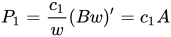
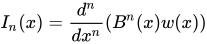When $n=0$, it is trivial. When $n=1$, it simplifies to $AP_{1}'=A'P_{1}$, which is true since $P_{1}={\frac {c_{1}}{w}}(Bw)'=c_{1}A$. So assume $n\geq 2$. Define $I_{n}(x)={\frac {d^{n}}{dx^{n}}}(B^{n}(x)w(x))$, then by direct computation and simplification, the equation to be proven is equivalent to

$${\frac {d^{2}}{dx^{2}}}(B(x)I_{n}(x))-{\frac {d}{dx}}(A(x)I_{n}(x))+\lambda _{n}I_{n}(x)=0$$

By Leibniz differentiation rule, we have

$$B(x){\frac {d^{n}}{dx^{n}}}y={\frac {d^{n}}{dx^{n}}}(B(x)y)-n{\frac {d^{n-1}}{dx^{n-1}}}(B'(x)y)+{\frac {n(n-1)}{2}}{\frac {d^{n-2}}{dx^{n-2}}}(B''y)$$

$$A(x){\frac {d^{n}}{dx^{n}}}y={\frac {d^{n}}{dx^{n}}}(A(x)y)-n{\frac {d^{n-1}}{dx^{n-1}}}(A'y)$$

for arbitrary $y$. This allows us to move $A(x),B(x)$ to the other side of the $n$-th derivative. Set $y=B^{n}(x)w(x)$, and define

$$J(x)={\frac {d^{2}}{dx^{2}}}(B(x)y(x))-n{\frac {d}{dx}}(B'(x)y(x))+{\frac {n(n-1)}{2}}B''y(x)$$

$$K(x)=-{\frac {d}{dx}}(A(x)y(x))+nA'y(x)$$

$$L(x)=\lambda _{n}y(x)$$

Then the equation simplifies to ${\frac {d^{n}}{dx^{n}}}(J+K+L)=0$

$J(x)$ has three terms, call them in order $J_{1}(x),J_{2}(x),J_{3}(x)$. $K(x)$ has two terms, call them in order $K_{1}(x),K_{2}(x)$.

$J_{3}(x)+K_{2}(x)+L(x)=(\lambda _{n}+{\frac {n(n-1)}{2}}B''+nA')y=0$.

That $J_{1}(x)+J_{2}(x)+K_{1}(x)=0$. follows from first writing $J_{1}(x)$ as

$J_{1}(x)={\frac {d^{2}}{dx^{2}}}\left(B^{n}(x)\int \exp \left({\frac {A(x)}{B(x)}}\right)dx\right)$

and then taking the innermost first derivative to obtain

$J_{1}(x)={\frac {d}{dx}}\left[{\bigg (}nB'(x)B^{n-1}(x)+A(x)B^{n-1}(x){\bigg )}\int \exp \left({\frac {A(x)}{B(x)}}\right)dx\right]$

and then rewriting this as

$J_{1}(x)={\frac {d}{dx}}{\Big (}nB'(x)B^{n}(x)w(x)+A(x)B^{n}(x)w(x){\Big )}$

The first term is the negative of $J_{2}(x)$ and the second term is the negative of $K_{1}(x)$.

More abstractly, this can be viewed through Sturm–Liouville theory. Define an operator $Lf:=-{\frac {1}{w}}(Wf')'$, then the differential equation is equivalent to $LP_{n}=\lambda _{n}P_{n}$. Define the functional space $X=L^{2}([a,b],w(x)dx)$ as the Hilbert space of functions over $[a,b]$, such that ${\displays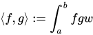tyle \langle f,g\rangle$ :=\int _{a}^{b}fgw} . Then the operator $L$ is self-adjoint on functions satisfying certain boundary conditions, allowing us to apply the spectral theorem.

Generating function

A simple argument using Cauchy's integral formula shows that the orthogonal polynomials obtained from the Rodrigues formula have a generating function of the form

$G(x,u)=\sum _{n=0}^{\infty }u^{n}P_{n}(x)$

The $P_{n}(x)$ functions here may not have the standard normalizations. But we can write this equivalently as

$G(x,u)=\sum _{n=0}^{\infty }{\frac {u^{n}}{N_{n}}}N_{n}P_{n}(x)$

where the $N_{n}$ are chosen according to the application so as to give the desired normalizations. The variable u may be replaced by a constant multiple of u so that

$G(x,\alpha u)=\sum _{n=0}^{\infty }{\frac {\alpha ^{n}u^{n}}{N_{n}}}N_{n}P_{n}(x)$

This gives an alternate form of the generating function.

By Cauchy's integral formula, Rodrigues’ formula is equivalent to$$P_{n}(x)={\frac {n!}{2\pi i}}{\frac {c_{n}}{w(x)}}\oint _{C}{\frac {B^{n}(t)w(t)}{(t-x)^{n+1}}}\,dt$$where the integral is along a counterclockwise closed loop around $x$. Let

$u={\frac {t-x}{B(t)}}$

Then the complex path integral takes the form

$P_{n}(x)={\frac {n!}{2\pi i}}c_{n}\oint _{C}{\frac {G(x,u)}{u^{n+1}}}\,du$

$G(x,u)={\frac {w(t){\frac {dt}{du}}}{w(x)B(t)}}$

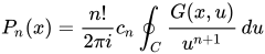
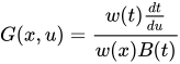
where now the closed path C encircles the origin. In the equation for $G(x,u)$, $t$ is an implicit function of $u$. Expanding $G(x,u)$ in the power series given earlier gives

${\frac {1}{2\pi i}}\oint _{C}{\frac {G(x,u)}{u^{n+1}}}\,du={\frac {1}{2\pi i}}\oint _{C}{\frac {\sum _{m=0}^{\infty }u^{m}P_{m}(x)}{u^{n+1}}}\,du=P_{n}(x)$

Only the $m=n$ term has a nonzero residue, which is $P_{n}(x)$. The $n!\,c_{n}$ coefficient was dropped since normalizations are conventions which can be inserted afterwards as discussed earlier.

By expressing t in terms of u in the general formula just given for $G(x,u)$, explicit formulas for $G(x,u)$ may be found. As a simple example, let $B(x)=1$ and $A(x)=-x$ (Hermite polynomials) so that $w(x)=\exp \left(-{\frac {x^{2}}{2}}\right)$, $t=u+x$, $w(t)=\exp \left(-{\frac {(u+x)^{2}}{2}}\right)$ and so $G(x,u)=\exp \left(-xu-{\frac {u^{2}}{2}}\right)$.

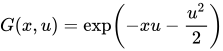Examples

Family	$[a,b]$	$w$	$W$	$A$	$B$	$c_{n}$
Legendre $P_{n}$	$[-1,+1]$	$1$	$1-x^{2}$	$-2x$	$1-x^{2}$	${\frac {(-1)^{n}}{2^{n}n!}}$
Chebyshev (of the first kind) $T_{n}$	$[-1,+1]$	$1/{\sqrt {1-x^{2}}}$	${\sqrt {1-x^{2}}}$	$-x$	$1-x^{2}$	${\frac {(-1)^{n}}{(2n-1)!!}}$
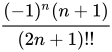
Chebyshev (of the second kind) $U_{n}$	$[-1,+1]$	${\sqrt {1-x^{2}}}$	$(1-x^{2})^{3/2}$	$-3x$	$1-x^{2}$	${\frac {(-1)^{n}(n+1)}{(2n+1)!!}}$
Gegenbauer/ultraspherical $C_{n}^{(\alpha )}(x)$	$[-1,+1]$	$(1-x)^{\alpha -1/2}(1+x)^{\alpha -1/2}$	$(1-x)^{\alpha +1/2}(1+x)^{\alpha +1/2}$	$-(2\alpha +1)x$	$1-x^{2}$	${\frac {(-1)^{n}(2\alpha )_{n}}{(\alpha +{\frac {1}{2}})_{n}2^{n}n!}}$
Jacobi $P_{n}^{(\alpha ,\beta )}$	$[-1,+1]$	$(1-x)^{\alpha }(1+x)^{\beta }$	$(1-x)^{\alpha +1}(1+x)^{\beta +1}$	$(\beta -\alpha )-(\alpha +\beta +2)x$	$1-x^{2}$	${\frac {(-1)^{n}}{2^{n}n!}}$
associated Laguerre $L_{n}^{(\alpha )}$	$[0,\infty )$	$x^{\alpha }e^{-x}$	$x^{\alpha +1}e^{-x}$	$\alpha +1-x$	$x$	${\frac {1}{n!}}$
physicist's Hermite $H_{n}$	$(-\infty ,+\infty )$	$e^{-x^{2}}$	$e^{-x^{2}}$	$-2x$	$1$	$(-1)^{n}$

These formulae are for the classical orthogonal polynomials. Similar formulae hold for many other sequences of orthogonal functions arising from Sturm–Liouville equations, and these are also called the Rodrigues formula (or Rodrigues' type formula), especially when the resulting sequence is polynomial.

Legendre

Source:

Rodrigues stated his formula for Legendre polynomials $P_{n}$:

$$P_{n}(x)={\frac {1}{2^{n}n!}}{\frac {d^{n}}{dx^{n}}}\!\left[(x^{2}-1)^{n}\right]\!.$$ $$(1-x^{2})P_{n}''(x)-2xP_{n}'(x)+n(n+1)P_{n}(x)=0$$

For Legendre polynomials, the generating function is defined as

$G(x,u)=\sum _{n=0}^{\infty }u^{n}P_{n}(x)$.

The contour integral gives the Schläfli integral for Legendre polynomials:

$$P_{n}(x)={\frac {1}{2\pi i2^{n}}}\oint _{C}{\frac {(t^{2}-1)^{n}}{(t-x)^{n+1}}}dt$$

Summing up the integrand

$$G(x,u)={\frac {1}{\sqrt {1-2ux+u^{2}}}}{\frac {1}{2\pi i}}\oint _{C}\left({\frac {1}{t-t_{-}}}-{\frac {1}{t-t_{+}}}\right)dt$$

where $t_{\pm }={\frac {1}{u}}(1\pm {\sqrt {1-2ux+u^{2}}})$. For small $u$, we have $t_{-}\approx x,t_{+}\to \infty$, which heuristically suggests that the integral should be the residue around $t_{-}$, thus giving

$$G(x,u)={\frac {1}{\sqrt {1-2ux+u^{2}}}}$$

Hermite

Source:

Physicist's Hermite polynomials:

$$H_{n}(x)=(-1)^{n}e^{x^{2}}{\frac {d^{n}}{dx^{n}}}\!\left[e^{-x^{2}}\right]=\left(2x-{\frac {d}{dx}}\right)^{n}\cdot 1.$$$$H_{n}''-2xH_{n}'+2nH_{n}=0$$

The generating function is defined as

$$G(x,u)=\sum _{n=0}^{\infty }{\frac {H_{n}(x)}{n!}}\,u^{n}.$$

The contour integral gives

$$H_{n}(x)=(-1)^{n}e^{x^{2}}{\frac {n!}{2\pi i}}\oint _{C}{\frac {e^{-t^{2}}}{(t-x)^{n+1}}}\,dt.$$

$${\begin{aligned}G(x,u)&=\sum _{n=0}^{\infty }{\frac {(-1)^{n}e^{x^{2}}}{n!}}{\frac {n!}{2\pi i}}\,u^{n}\oint _{C}{\frac {e^{-t^{2}}}{(t-x)^{n+1}}}\,dt\\&=e^{x^{2}}{\frac {1}{2\pi i}}\oint _{C}e^{-t^{2}}\left(\sum _{n=0}^{\infty }{\frac {(-1)^{n}u^{n}}{(t-x)^{n+1}}}\right)dt\\&=e^{x^{2}}{\frac {1}{2\pi i}}\oint _{C}e^{-t^{2}}{\frac {1}{t-x+u}}\\&=e^{x^{2}}\,e^{-(x-u)^{2}}\\&=e^{2xu-u^{2}}\end{aligned}}$$

Laguerre

Source:

For associated Laguerre polynomials

$$L_{n}^{(\alpha )}(x)={x^{-\alpha }e^{x} \over n!}{d^{n} \over dx^{n}}\left(e^{-x}x^{n+\alpha }\right)={\frac {x^{-\alpha }}{n!}}\left({\frac {d}{dx}}-1\right)^{n}x^{n+\alpha }.$$

$$xL_{n}^{(\alpha )}(x)''+(\alpha +1-x)L_{n}^{(\alpha )}(x)'+nL_{n}^{(\alpha )}(x)=0~.$$

The generating function is defined as

$$G(x,u):=\sum _{n=0}^{\infty }u^{n}L_{n}^{(\alpha )}(x)$$

By the same method, we have $G(x,u)={\frac {1}{(1-u)^{\alpha +1}}}e^{-{\frac {ux}{1-u}}}$.

Jacobi

Source:

$$P_{n}^{(\alpha ,\beta )}(x)={\frac {(-1)^{n}}{2^{n}n!}}(1-x)^{-\alpha }(1+x)^{-\beta }{\frac {d^{n}}{dx^{n}}}\left\{(1-x)^{\alpha }(1+x)^{\beta }\left(1-x^{2}\right)^{n}\right\}.$$$$\left(1-x^{2}\right)P_{n}^{(\alpha ,\beta )}{}''+(\beta -\alpha -(\alpha +\beta +2)x)P_{n}^{(\alpha ,\beta )}{}'+n(n+\alpha +\beta +1)P_{n}^{(\alpha ,\beta )}=0.$$

$\sum _{n=0}^{\infty }P_{n}^{(\alpha ,\beta )}(x)u^{n}=2^{\alpha +\beta }R^{-1}(1-u+R)^{-\alpha }(1+u+R)^{-\beta },$

where ${\textstyle R={\sqrt {1-2ux+u^{2}}}}$, and the branch of square root is chosen so that $R(x,0)=1$.

See also

• Classical orthogonal polynomials

References

• Askey, Richard (2005), "The 1839 paper on permutations: its relation to the Rodrigues formula and further developments", in Altmann, Simón L.; Ortiz, Eduardo L. (eds.), Mathematics and social utopias in France: Olinde Rodrigues and his times, History of mathematics, vol. 28, Providence, R.I.: American Mathematical Society, pp. 105–118, ISBN 978-0-8218-3860-0
• Ivory, James (1824), "On the Figure Requisite to Maintain the Equilibrium of a Homogeneous Fluid Mass That Revolves Upon an Axis", Philosophical Transactions of the Royal Society of London, 114, The Royal Society: 85–150, doi:10.1098/rstl.1824.0008, JSTOR 107707
• Jacobi, C. G. J. (1827), "Ueber eine besondere Gattung algebraischer Functionen, die aus der Entwicklung der Function (1 − 2xz + z²)^1/2 entstehen.", Journal für die Reine und Angewandte Mathematik (in German), 2: 223–226, doi:10.1515/crll.1827.2.223, ISSN 0075-4102, S2CID 120291793
• O'Connor, John J.; Robertson, Edmund F., "Olinde Rodrigues", MacTutor History of Mathematics Archive, University of St Andrews
• Rodrigues, Olinde (1816), "De l'attraction des sphéroïdes", Correspondence sur l'École Impériale Polytechnique, (Thesis for the Faculty of Science of the University of Paris), 3 (3): 361–385