Newman–Penrose formalism

The Newman–Penrose (NP) formalism is a set of notation developed by Ezra T. Newman and Roger Penrose for general relativity (GR). Their notation is an effort to treat general relativity in terms of spinor notation, which introduces complex forms of the usual variables used in GR. The NP formalism is itself a special case of the tetrad formalism, where the tensors of the theory are projected onto a complete vector basis at each point in spacetime. Usually this vector basis is chosen to reflect some symmetry of the spacetime, leading to simplified expressions for physical observables. In the case of the NP formalism, the vector basis chosen is a null tetrad: a set of four null vectors—two real, and a complex-conjugate pair. The two real members often asymptotically point radially inward and radially outward, and the formalism is well adapted to treatment of the propagation of radiation in curved spacetime. The Weyl scalars, derived from the Weyl tensor, are often used. In particular, it can be shown that one of these scalars—$\Psi _{4}$ in the appropriate frame—encodes the outgoing gravitational radiation of an asymptotically flat system.

Newman and Penrose introduced the following functions as primary quantities using this tetrad:

• Twelve complex spin coefficients (in three groups) which describe the change in the tetrad from point to point: $\kappa ,\rho ,\sigma ,\tau \,;\lambda ,\mu ,\nu ,\pi \,;\epsilon ,\gamma ,\beta ,\alpha .$.
• Five complex functions encoding Weyl tensors in the tetrad basis: $\Psi _{0},\ldots ,\Psi _{4}$.
• Ten functions encoding Ricci tensors in the tetrad basis: $\Phi _{00},\Phi _{11},\Phi _{22},\Lambda$ (real); $\Phi _{01},\Phi _{10},\Phi _{02},\Phi _{20},\Phi _{12},\Phi _{21}$ (complex).

In many situations—especially algebraically special spacetimes or vacuum spacetimes—the Newman–Penrose formalism simplifies dramatically, as many of the functions go to zero. This simplification allows for various theorems to be proven more easily than using the standard form of Einstein's equations.

In this article, we will only employ the tensorial rather than spinorial version of NP formalism, because the former is easier to understand and more popular in relevant papers. One can refer to ref. for a unified formulation of these two versions.

Null tetrad and sign convention

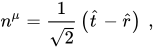
The formalism is developed for four-dimensional spacetime, with a Lorentzian-signature metric. At each point, a tetrad (set of four vectors) is introduced. The first two vectors, $\ell ^{\mu }$ and $n^{\mu }$ are just a pair of standard (real) null vectors such that $\ell ^{a}n_{a}=-1$. For example, we can think in terms of spherical coordinates, and take $\ell ^{a}$ to be the outgoing null vector, and $n^{a}$ to be the ingoing null vector. A complex null vector is then constructed by combining a pair of real, orthogonal unit space-like vectors. In the case of spherical coordinates, the standard choice is $$m^{\mu }={\frac {1}{\sqrt {2}}}\left({\hat {\theta }}+i{\hat {\phi }}\right)^{\mu }\ .$$ The complex conjugate of this vector then forms the fourth element of the tetrad.

Two sets of signature and normalization conventions are in use for NP formalism: $\{(+,-,-,-);\ell ^{a}n_{a}=1\,,m^{a}{\bar {m}}_{a}=-1\}$ and $\{(-,+,+,+);\ell ^{a}n_{a}=-1\,,m^{a}{\bar {m}}_{a}=1\}$. The former is the original one that was adopted when NP formalism was developed and has been widely used in black-hole physics, gravitational waves and various other areas in general relativity. However, it is the latter convention that is usually employed in contemporary study of black holes from quasilocal perspectives (such as isolated horizons and dynamical horizons). In this article, we will utilize $\{(-,+,+,+);\ell ^{a}n_{a}=-1\,,m^{a}{\bar {m}}_{a}=1\}$ for a systematic review of the NP formalism (see also refs.).

It's important to note that, when switching from $\{(+,-,-,-)\,,\ell ^{a}n_{a}=1\,,m^{a}{\bar {m}}_{a}=-1\}$ to $\{(-,+,+,+)\,,\ell ^{a}n_{a}=-1\,,m^{a}{\bar {m}}_{a}=1\}$, definitions of the spin coefficients, Weyl-NP scalars $\Psi _{i}$ and Ricci-NP scalars $\Phi _{ij}$ need to change their signs; this way, the Einstein-Maxwell equations can be left unchanged.

In NP formalism, the complex null tetrad contains two real null (co)vectors $\{\ell \,,n\}$ and two complex null (co)vectors $\{m\,,{\bar {m}}\}$. Being null (co)vectors, self-normalization of $\{\ell \,,n\}$ naturally vanishes,

$$\ell _{a}\ell ^{a}=n_{a}n^{a}=m_{a}m^{a}={\bar {m}}_{a}{\bar {m}}^{a}=0,$$

so the following two pairs of cross-normalization are adopted

$$\ell _{a}n^{a}=-1=\ell ^{a}n_{a}\,,\quad m_{a}{\bar {m}}^{a}=1=m^{a}{\bar {m}}_{a}\,,$$

while contractions between the two pairs are also vanishing,

$$\ell _{a}m^{a}=\ell _{a}{\bar {m}}^{a}=n_{a}m^{a}=n_{a}{\bar {m}}^{a}=0.$$

Here the indices can be raised and lowered by the global metric $g_{ab}$ which in turn can be obtained via

$${\begin{aligned}g_{ab}&=-\ell _{a}n_{b}-n_{a}\ell _{b}+m_{a}{\bar {m}}_{b}+{\bar {m}}_{a}m_{b}\,,\\[1ex]g^{ab}&=-\ell ^{a}n^{b}-n^{a}\ell ^{b}+m^{a}{\bar {m}}^{b}+{\bar {m}}^{a}m^{b}\,.\end{aligned}}$$

NP quantities and tetrad equations

Four covariant derivative operators

In keeping with the formalism's practice of using distinct unindexed symbols for each component of an object, the covariant derivative operator $\nabla _{a}$ is expressed using four separate symbols ($D,\Delta ,\delta ,{\bar {\delta }}$) which name a directional covariant derivative operator for each tetrad direction. Given a linear combination of tetrad vectors, $X^{a}=\mathrm {a} \ell ^{a}+\mathrm {b} n^{a}+\mathrm {c} m^{a}+\mathrm {d} {\bar {m}}^{a}$, the covariant derivative operator in the $X^{a}$ direction is $\nabla _{X}=X^{a}\nabla _{a}=(\mathrm {a} D+\mathrm {b} \Delta +\mathrm {c} \delta +\mathrm {d} {\bar {\delta }})$.

The operators are defined as

$${\begin{aligned}D&:=\nabla _{\boldsymbol {\ell }}=\ell ^{a}\nabla _{a}\,,&\Delta &:=\nabla _{\boldsymbol {n}}=n^{a}\nabla _{a}\,,\\[1ex]\delta &:=\nabla _{\boldsymbol {m}}=m^{a}\nabla _{a}\,,&{\bar {\delta }}&:=\nabla _{\boldsymbol {\bar {m}}}={\bar {m}}^{a}\nabla _{a}\,,\end{aligned}}$$

which reduce to $D=\ell ^{a}\partial _{a}\,,\Delta =n^{a}\partial _{a}\,,\delta =m^{a}\partial _{a}\,,{\bar {\delta }}={\bar {m}}^{a}\partial _{a}$ when acting on scalar functions.

Twelve spin coefficients

In NP formalism, instead of using index notations as in orthogonal tetrads, each Ricci rotation coefficient $\gamma _{ijk}$ in the null tetrad is assigned a lower-case Greek letter, which constitute the 12 complex spin coefficients (in three groups),

$${\begin{aligned}\kappa &:=-m^{a}D\ell _{a}=-m^{a}\ell ^{b}\nabla _{b}\ell _{a}\,,&\tau &:=-m^{a}\Delta \ell _{a}=-m^{a}n^{b}\nabla _{b}\ell _{a}\,,\\[1ex]\sigma &:=-m^{a}\delta \ell _{a}=-m^{a}m^{b}\nabla _{b}\ell _{a}\,,&\rho &:=-m^{a}{\bar {\delta }}\ell _{a}=-m^{a}{\bar {m}}^{b}\nabla _{b}\ell _{a}\,;\\[1ex]\pi &:={\bar {m}}^{a}Dn_{a}={\bar {m}}^{a}\ell ^{b}\nabla _{b}n_{a}\,,&\nu &:={\bar {m}}^{a}\Delta n_{a}={\bar {m}}^{a}n^{b}\nabla _{b}n_{a}\,,\\[1ex]\mu &:={\bar {m}}^{a}\delta n_{a}={\bar {m}}^{a}m^{b}\nabla _{b}n_{a}\,,&\lambda &:={\bar {m}}^{a}{\bar {\delta }}n_{a}={\bar {m}}^{a}{\bar {m}}^{b}\nabla _{b}n_{a}\,;\end{aligned}}$$ $${\begin{aligned}\varepsilon &:=-{\tfrac {1}{2}}\left(n^{a}D\ell _{a}-{\bar {m}}^{a}Dm_{a}\right)=-{\tfrac {1}{2}}\left(n^{a}\ell ^{b}\nabla _{b}\ell _{a}-{\bar {m}}^{a}\ell ^{b}\nabla _{b}m_{a}\right)\,,\\[1ex]\gamma &:=-{\tfrac {1}{2}}\left(n^{a}\Delta \ell _{a}-{\bar {m}}^{a}\Delta m_{a}\right)=-{\tfrac {1}{2}}\left(n^{a}n^{b}\nabla _{b}\ell _{a}-{\bar {m}}^{a}n^{b}\nabla _{b}m_{a}\right)\,,\\[1ex]\beta &:=-{\tfrac {1}{2}}\left(n^{a}\delta \ell _{a}-{\bar {m}}^{a}\delta m_{a}\right)=-{\tfrac {1}{2}}\left(n^{a}m^{b}\nabla _{b}\ell _{a}-{\bar {m}}^{a}m^{b}\nabla _{b}m_{a}\right)\,,\\[1ex]\alpha &:=-{\tfrac {1}{2}}\left(n^{a}{\bar {\delta }}\ell _{a}-{\bar {m}}^{a}{\bar {\delta }}m_{a}\right)=-{\tfrac {1}{2}}\left(n^{a}{\bar {m}}^{b}\nabla _{b}\ell _{a}-{\bar {m}}^{a}{\bar {m}}^{b}\nabla _{b}m_{a}\right)\,.\end{aligned}}$$

Spin coefficients are the primary quantities in NP formalism, with which all other NP quantities (as defined below) could be calculated indirectly using the NP field equations. Thus, NP formalism is sometimes referred to as spin-coefficient formalism as well.

Transportation equations: covariant derivatives of tetrad vectors

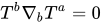
The sixteen directional covariant derivatives of tetrad vectors are sometimes called the transportation/propagation equations, perhaps because the derivatives are zero when the tetrad vector is parallel propagated or transported in the direction of the derivative operator.

These results in this exact notation are given by O'Donnell: $${\begin{aligned}D\ell ^{a}&=\left(\varepsilon +{\bar {\varepsilon }}\right)\ell ^{a}-{\bar {\kappa }}m^{a}-\kappa {\bar {m}}^{a}\,,\\[1ex]\Delta \ell ^{a}&=\left(\gamma +{\bar {\gamma }}\right)\ell ^{a}-{\bar {\tau }}m^{a}-\tau {\bar {m}}^{a}\,,\\[1ex]\delta \ell ^{a}&=\left({\bar {\alpha }}+\beta \right)\ell ^{a}-{\bar {\rho }}m^{a}-\sigma {\bar {m}}^{a}\,,\\[1ex]{\bar {\delta }}\ell ^{a}&=\left(\alpha +{\bar {\beta }}\right)\ell ^{a}-{\bar {\sigma }}m^{a}-\rho {\bar {m}}^{a}\,;\end{aligned}}$$ $${\begin{aligned}Dn^{a}&=\pi m^{a}+{\bar {\pi }}{\bar {m}}^{a}-\left(\varepsilon +{\bar {\varepsilon }}\right)n^{a}\,,\\[1ex]\Delta n^{a}&=\nu m^{a}+{\bar {\nu }}{\bar {m}}^{a}-\left(\gamma +{\bar {\gamma }}\right)n^{a}\,,\\[1ex]\delta n^{a}&=\mu m^{a}+{\bar {\lambda }}{\bar {m}}^{a}-\left({\bar {\alpha }}+\beta \right)n^{a}\,,\\[1ex]{\bar {\delta }}n^{a}&=\lambda m^{a}+{\bar {\mu }}{\bar {m}}^{a}-\left(\alpha +{\bar {\beta }}\right)n^{a}\,;\end{aligned}}$$ $${\begin{aligned}Dm^{a}&=\left(\varepsilon -{\bar {\varepsilon }}\right)m^{a}+{\bar {\pi }}\ell ^{a}-\kappa n^{a}\,,\\[1ex]\Delta m^{a}&=\left(\gamma -{\bar {\gamma }}\right)m^{a}+{\bar {\nu }}\ell ^{a}-\tau n^{a}\,,\\[1ex]\delta m^{a}&=\left(\beta -{\bar {\alpha }}\right)m^{a}+{\bar {\lambda }}\ell ^{a}-\sigma n^{a}\,,\\[1ex]{\bar {\delta }}m^{a}&=\left(\alpha -{\bar {\beta }}\right)m^{a}+{\bar {\mu }}\ell ^{a}-\rho n^{a}\,;\end{aligned}}$$ $${\begin{aligned}D{\bar {m}}^{a}&=\left({\bar {\varepsilon }}-\varepsilon \right){\bar {m}}^{a}+\pi \ell ^{a}-{\bar {\kappa }}n^{a}\,,\\[1ex]\Delta {\bar {m}}^{a}&=\left({\bar {\gamma }}-\gamma \right){\bar {m}}^{a}+\nu \ell ^{a}-{\bar {\tau }}n^{a}\,,\\[1ex]\delta {\bar {m}}^{a}&=\left({\bar {\alpha }}-\beta \right){\bar {m}}^{a}+\mu \ell ^{a}-{\bar {\rho }}n^{a}\,,\\[1ex]{\bar {\delta }}{\bar {m}}^{a}&=\left({\bar {\beta }}-\alpha \right){\bar {m}}^{a}+\lambda \ell ^{a}-{\bar {\sigma }}n^{a}\,.\end{aligned}}$$

Interpretation of κ, ε, ν, γ from Dℓ^a and Δn^a

The two equations for the covariant derivative of a real null tetrad vector in its own direction indicate whether or not the vector is tangent to a geodesic and if so, whether the geodesic has an affine parameter.

A null tangent vector $T^{a}$ is tangent to an affinely parameterized null geodesic if $T^{b}\nabla _{b}T^{a}=0$, which is to say if the vector is unchanged by parallel propagation or transportation in its own direction.

$D\ell ^{a}=(\varepsilon +{\bar {\varepsilon }})\ell ^{a}-{\bar {\kappa }}m^{a}-\kappa {\bar {m}}^{a}$ shows that $\ell ^{a}$ is tangent to a geodesic if and only if $\kappa =0$, and is tangent to an affinely parameterized geodesic if in addition $(\varepsilon +{\bar {\varepsilon }})=0$. Similarly, $\Delta n^{a}=\nu m^{a}+{\bar {\nu }}{\bar {m}}^{a}-(\gamma +{\bar {\gamma }})n^{a}$ shows that $n^{a}$ is geodesic if and only if $\nu =0$, and has affine parameterization when $(\gamma +{\bar {\gamma }})=0$.

(The complex null tetrad vectors $m^{a}=x^{a}+iy^{a}$ and ${\bar {m}}^{a}=x^{a}-iy^{a}$ would have to be separated into the spacelike basis vectors $x^{a}$ and $y^{a}$ before asking if either or both of those are tangent to spacelike geodesics.)

Commutators

The metric-compatibility or torsion-freeness of the covariant derivative is recast into the commutators of the directional derivatives,

$${\begin{aligned}\Delta D-D\Delta &=\left(\gamma +{\bar {\gamma }}\right)D+\left(\varepsilon +{\bar {\varepsilon }}\right)\Delta -\left({\bar {\tau }}+\pi \right)\delta -\left(\tau +{\bar {\pi }}\right){\bar {\delta }}\,,\\[1ex]\delta D-D\delta &=\left({\bar {\alpha }}+\beta -{\bar {\pi }}\right)D+\kappa \Delta -\left({\bar {\rho }}+\varepsilon -{\bar {\varepsilon }}\right)\delta -\sigma {\bar {\delta }}\,,\\[1ex]\delta \Delta -\Delta \delta &=-{\bar {\nu }}D+\left(\tau -{\bar {\alpha }}-\beta \right)\Delta +\left(\mu -\gamma +{\bar {\gamma }}\right)\delta +{\bar {\lambda }}{\bar {\delta }}\,,\\[1ex]{\bar {\delta }}\delta -\delta {\bar {\delta }}&=\left({\bar {\mu }}-\mu \right)D+\left({\bar {\rho }}-\rho \right)\Delta +\left(\alpha -{\bar {\beta }}\right)\delta -\left({\bar {\alpha }}-\beta \right){\bar {\delta }}\,,\end{aligned}}$$

which imply that

$${\begin{aligned}\Delta \ell ^{a}-Dn^{a}&=\left(\gamma +{\bar {\gamma }}\right)\ell ^{a}+\left(\varepsilon +{\bar {\varepsilon }}\right)n^{a}-\left({\bar {\tau }}+\pi \right)m^{a}-\left(\tau +{\bar {\pi }}\right){\bar {m}}^{a}\,,\\[1ex]\delta \ell ^{a}-Dm^{a}&=\left({\bar {\alpha }}+\beta -{\bar {\pi }}\right)\ell ^{a}+\kappa n^{a}-\left({\bar {\rho }}+\varepsilon -{\bar {\varepsilon }}\right)m^{a}-\sigma {\bar {m}}^{a}\,,\\[1ex]\delta n^{a}-\Delta m^{a}&=-{\bar {\nu }}\ell ^{a}+\left(\tau -{\bar {\alpha }}-\beta \right)n^{a}+\left(\mu -\gamma +{\bar {\gamma }}\right)m^{a}+{\bar {\lambda }}{\bar {m}}^{a}\,,\\[1ex]{\bar {\delta }}m^{a}-\delta {\bar {m}}^{a}&=\left({\bar {\mu }}-\mu \right)\ell ^{a}+\left({\bar {\rho }}-\rho \right)n^{a}+\left(\alpha -{\bar {\beta }}\right)m^{a}-\left({\bar {\alpha }}-\beta \right){\bar {m}}^{a}\,.\end{aligned}}$$

Note: (i) The above equations can be regarded either as implications of the commutators or combinations of the transportation equations; (ii) In these implied equations, the vectors $\{\ell ^{a},n^{a},m^{a},{\bar {m}}^{a}\}$ can be replaced by the covectors and the equations still hold.

Weyl–NP and Ricci–NP scalars

The 10 independent components of the Weyl tensor can be encoded into 5 complex Weyl-NP scalars,

$${\begin{aligned}\Psi _{0}&:=C_{abcd}\ell ^{a}m^{b}\ell ^{c}m^{d}\,,&\Psi _{1}&:=C_{abcd}\ell ^{a}n^{b}\ell ^{c}m^{d}\,,\\\Psi _{2}&:=C_{abcd}\ell ^{a}m^{b}{\bar {m}}^{c}n^{d}\,,&\Psi _{3}&:=C_{abcd}\ell ^{a}n^{b}{\bar {m}}^{c}n^{d}\,,\\\Psi _{4}&:=C_{abcd}n^{a}{\bar {m}}^{b}n^{c}{\bar {m}}^{d}\,.\end{aligned}}$$

The 10 independent components of the Ricci tensor are encoded into 4 real scalars $\{\Phi _{00}$, $\Phi _{11}$, $\Phi _{22}$, $\Lambda \}$ and 3 complex scalars $\{\Phi _{10},\Phi _{20},\Phi _{21}\}$ (with their complex conjugates),

$${\begin{aligned}\Phi _{00}&:={\tfrac {1}{2}}R_{ab}\ell ^{a}\ell ^{b}\,,&\Phi _{11}&:={\tfrac {1}{4}}R_{ab}\left(\ell ^{a}n^{b}+m^{a}{\bar {m}}^{b}\right),\\[1ex]\Phi _{22}&:={\tfrac {1}{2}}R_{ab}n^{a}n^{b}\,,&\Lambda &:={\tfrac {1}{24}}R\,;\end{aligned}}$$$${\begin{aligned}\Phi _{01}&:={\tfrac {1}{2}}R_{ab}\ell ^{a}m^{b}\,,&\Phi _{10}&:={\tfrac {1}{2}}R_{ab}\ell ^{a}{\bar {m}}^{b}={\overline {\Phi _{01}}}\,,\\\Phi _{02}&:={\tfrac {1}{2}}R_{ab}m^{a}m^{b}\,,&\Phi _{20}&:={\tfrac {1}{2}}R_{ab}{\bar {m}}^{a}{\bar {m}}^{b}={\overline {\Phi _{02}}}\,,\\\Phi _{12}&:={\tfrac {1}{2}}R_{ab}m^{a}n^{b}\,,&\Phi _{21}&:={\tfrac {1}{2}}R_{ab}{\bar {m}}^{a}n^{b}={\overline {\Phi _{12}}}\,.\end{aligned}}$$

In these definitions, $R_{ab}$ could be replaced by its trace-free part ${\textstyle Q_{ab}=R_{ab}-{\tfrac {1}{4}}g_{ab}R}$ or by the Einstein tensor ${\textstyle G_{ab}=R_{ab}-{\tfrac {1}{2}}g_{ab}R}$ because of the normalization relations. Also, $\Phi _{11}$ is reduced to ${\textstyle \Phi _{11}={\tfrac {1}{2}}R_{ab}\ell ^{a}n^{b}={\tfrac {1}{2}}R_{ab}m^{a}{\bar {m}}^{b}}$ for electrovacuum ($\Lambda =0$).

Einstein–Maxwell–NP equations

NP field equations

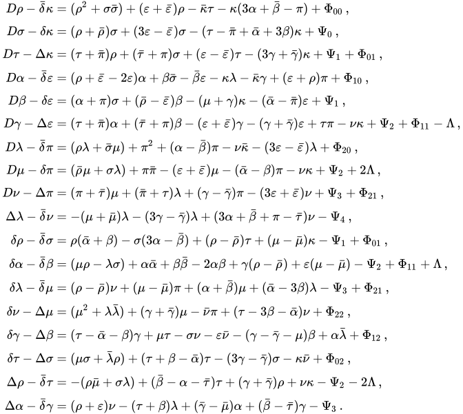
In a complex null tetrad, Ricci identities give rise to the following NP field equations connecting spin coefficients, Weyl-NP and Ricci-NP scalars (recall that in an orthogonal tetrad, Ricci rotation coefficients would respect Cartan's first and second structure equations),

These equations in various notations can be found in several texts. The notation in Frolov and Novikov is identical.

$${\begin{aligned}D\rho -{\bar {\delta }}\kappa &=(\rho ^{2}+\sigma {\bar {\sigma }})+(\varepsilon +{\bar {\varepsilon }})\rho -{\bar {\kappa }}\tau -\kappa (3\alpha +{\bar {\beta }}-\pi )+\Phi _{00}\,,\\[1ex]D\sigma -\delta \kappa &=(\rho +{\bar {\rho }})\sigma +(3\varepsilon -{\bar {\varepsilon }})\sigma -(\tau -{\bar {\pi }}+{\bar {\alpha }}+3\beta )\kappa +\Psi _{0}\,,\\[1ex]D\tau -\Delta \kappa &=(\tau +{\bar {\pi }})\rho +({\bar {\tau }}+\pi )\sigma +(\varepsilon -{\bar {\varepsilon }})\tau -(3\gamma +{\bar {\gamma }})\kappa +\Psi _{1}+\Phi _{01}\,,\\[1ex]D\alpha -{\bar {\delta }}\varepsilon &=(\rho +{\bar {\varepsilon }}-2\varepsilon )\alpha +\beta {\bar {\sigma }}-{\bar {\beta }}\varepsilon -\kappa \lambda -{\bar {\kappa }}\gamma +(\varepsilon +\rho )\pi +\Phi _{10}\,,\\[1ex]D\beta -\delta \varepsilon &=(\alpha +\pi )\sigma +({\bar {\rho }}-{\bar {\varepsilon }})\beta -(\mu +\gamma )\kappa -({\bar {\alpha }}-{\bar {\pi }})\varepsilon +\Psi _{1}\,,\\[1ex]D\gamma -\Delta \varepsilon &=(\tau +{\bar {\pi }})\alpha +({\bar {\tau }}+\pi )\beta -(\varepsilon +{\bar {\varepsilon }})\gamma -(\gamma +{\bar {\gamma }})\varepsilon +\tau \pi -\nu \kappa +\Psi _{2}+\Phi _{11}-\Lambda \,,\\[1ex]D\lambda -{\bar {\delta }}\pi &=(\rho \lambda +{\bar {\sigma }}\mu )+\pi ^{2}+(\alpha -{\bar {\beta }})\pi -\nu {\bar {\kappa }}-(3\varepsilon -{\bar {\varepsilon }})\lambda +\Phi _{20}\,,\\[1ex]D\mu -\delta \pi &=({\bar {\rho }}\mu +\sigma \lambda )+\pi {\bar {\pi }}-(\varepsilon +{\bar {\varepsilon }})\mu -({\bar {\alpha }}-\beta )\pi -\nu \kappa +\Psi _{2}+2\Lambda \,,\\[1ex]D\nu -\Delta \pi &=(\pi +{\bar {\tau }})\mu +({\bar {\pi }}+\tau )\lambda +(\gamma -{\bar {\gamma }})\pi -(3\varepsilon +{\bar {\varepsilon }})\nu +\Psi _{3}+\Phi _{21}\,,\\[1ex]\Delta \lambda -{\bar {\delta }}\nu &=-(\mu +{\bar {\mu }})\lambda -(3\gamma -{\bar {\gamma }})\lambda +(3\alpha +{\bar {\beta }}+\pi -{\bar {\tau }})\nu -\Psi _{4}\,,\\[1ex]\delta \rho -{\bar {\delta }}\sigma &=\rho ({\bar {\alpha }}+\beta )-\sigma (3\alpha -{\bar {\beta }})+(\rho -{\bar {\rho }})\tau +(\mu -{\bar {\mu }})\kappa -\Psi _{1}+\Phi _{01}\,,\\[1ex]\delta \alpha -{\bar {\delta }}\beta &=(\mu \rho -\lambda \sigma )+\alpha {\bar {\alpha }}+\beta {\bar {\beta }}-2\alpha \beta +\gamma (\rho -{\bar {\rho }})+\varepsilon (\mu -{\bar {\mu }})-\Psi _{2}+\Phi _{11}+\Lambda \,,\\[1ex]\delta \lambda -{\bar {\delta }}\mu &=(\rho -{\bar {\rho }})\nu +(\mu -{\bar {\mu }})\pi +(\alpha +{\bar {\beta }})\mu +({\bar {\alpha }}-3\beta )\lambda -\Psi _{3}+\Phi _{21}\,,\\[1ex]\delta \nu -\Delta \mu &=(\mu ^{2}+\lambda {\bar {\lambda }})+(\gamma +{\bar {\gamma }})\mu -{\bar {\nu }}\pi +(\tau -3\beta -{\bar {\alpha }})\nu +\Phi _{22}\,,\\[1ex]\delta \gamma -\Delta \beta &=(\tau -{\bar {\alpha }}-\beta )\gamma +\mu \tau -\sigma \nu -\varepsilon {\bar {\nu }}-(\gamma -{\bar {\gamma }}-\mu )\beta +\alpha {\bar {\lambda }}+\Phi _{12}\,,\\[1ex]\delta \tau -\Delta \sigma &=(\mu \sigma +{\bar {\lambda }}\rho )+(\tau +\beta -{\bar {\alpha }})\tau -(3\gamma -{\bar {\gamma }})\sigma -\kappa {\bar {\nu }}+\Phi _{02}\,,\\[1ex]\Delta \rho -{\bar {\delta }}\tau &=-(\rho {\bar {\mu }}+\sigma \lambda )+({\bar {\beta }}-\alpha -{\bar {\tau }})\tau +(\gamma +{\bar {\gamma }})\rho +\nu \kappa -\Psi _{2}-2\Lambda \,,\\[1ex]\Delta \alpha -{\bar {\delta }}\gamma &=(\rho +\varepsilon )\nu -(\tau +\beta )\lambda +({\bar {\gamma }}-{\bar {\mu }})\alpha +({\bar {\beta }}-{\bar {\tau }})\gamma -\Psi _{3}\,.\end{aligned}}$$

Also, the Weyl-NP scalars $\Psi _{i}$ and the Ricci-NP scalars $\Phi _{ij}$ can be calculated indirectly from the above NP field equations after obtaining the spin coefficients rather than directly using their definitions.

Maxwell–NP scalars, Maxwell equations in NP formalism

The six independent components of the Faraday-Maxwell 2-form (i.e. the electromagnetic field strength tensor) $F_{ab}$ can be encoded into three complex Maxwell-NP scalars

$$\phi _{0}:=F_{ab}\ell ^{a}m^{b}\,,\quad \phi _{1}:={\tfrac {1}{2}}F_{ab}\left(\ell ^{a}n^{b}+{\bar {m}}^{a}m^{b}\right),\quad \phi _{2}:=F_{ab}{\bar {m}}^{a}n^{b}\,,$$

and therefore the eight real Maxwell equations $d\mathbf {F} =0$ and $d^{\star }\mathbf {F} =0$ (as $\mathbf {F} =dA$) can be transformed into four complex equations,

$${\begin{aligned}D\phi _{1}-{\bar {\delta }}\phi _{0}&=(\pi -2\alpha )\phi _{0}+2\rho \phi _{1}-\kappa \phi _{2}\,,\\[1ex]D\phi _{2}-{\bar {\delta }}\phi _{1}&=-\lambda \phi _{0}+2\pi \phi _{1}+(\rho -2\varepsilon )\phi _{2}\,,\\[1ex]\Delta \phi _{0}-\delta \phi _{1}&=(2\gamma -\mu )\phi _{0}-2\tau \phi _{1}+\sigma \phi _{2}\,,\\[1ex]\Delta \phi _{1}-\delta \phi _{2}&=\nu \phi _{0}-2\mu \phi _{1}+(2\beta -\tau )\phi _{2}\,,\end{aligned}}$$

with the Ricci-NP scalars $\Phi _{ij}$ related to Maxwell scalars by

$$\Phi _{ij}=\,2\,\phi _{i}\,{\overline {\phi _{j}}}\,,\quad (i,j\in \{0,1,2\})\,.$$

It is worthwhile to point out that, the supplementary equation $\Phi _{ij}=2\,\phi _{i}\,{\overline {\phi _{j}}}$ is only valid for electromagnetic fields; for example, in the case of Yang-Mills fields there will be $\Phi _{ij}=\,{\text{Tr}}\,(\digamma _{i}\,{\bar {\digamma }}_{j})$ where $\digamma _{i}(i\in \{0,1,2\})$ are Yang-Mills-NP scalars.

To sum up, the aforementioned transportation equations, NP field equations and Maxwell-NP equations together constitute the Einstein-Maxwell equations in Newman–Penrose formalism.

Applications of the NP formalism to gravitational radiation field

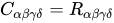
The Weyl scalar $\Psi _{4}$ was defined by Newman & Penrose as $$\Psi _{4}=-C_{\alpha \beta \gamma \delta }n^{\alpha }{\bar {m}}^{\beta }n^{\gamma }{\bar {m}}^{\delta }$$ (note, however, that the overall sign is arbitrary, and that Newman & Penrose worked with a "timelike" metric signature of $(+,-,-,-)$). In empty space, the Einstein field equations reduce to $R_{\alpha \beta }=0$. From the definition of the Weyl tensor, we see that this means that it equals the Riemann tensor, $C_{\alpha \beta \gamma \delta }=R_{\alpha \beta \gamma \delta }$. We can make the standard choice for the tetrad at infinity: $$\ell ^{\mu }={\frac {1}{\sqrt {2}}}\left({\hat {t}}+{\hat {r}}\right)\ ,$$ $$n^{\mu }={\frac {1}{\sqrt {2}}}\left({\hat {t}}-{\hat {r}}\right)\ ,$$ $$m^{\mu }={\frac {1}{\sqrt {2}}}\left({\hat {\theta }}+i{\hat {\phi }}\right)\ .$$

In transverse-traceless gauge, a simple calculation shows that linearized gravitational waves are related to components of the Riemann tensor as $${\tfrac {1}{4}}\left({\ddot {h}}_{{\hat {\theta }}{\hat {\theta }}}-{\ddot {h}}_{{\hat {\phi }}{\hat {\phi }}}\right)=-R_{{\hat {t}}{\hat {\theta }}{\hat {t}}{\hat {\theta }}}=-R_{{\hat {t}}{\hat {\phi }}{\hat {r}}{\hat {\phi }}}=-R_{{\hat {r}}{\hat {\theta }}{\hat {r}}{\hat {\theta }}}=R_{{\hat {t}}{\hat {\phi }}{\hat {t}}{\hat {\phi }}}=R_{{\hat {t}}{\hat {\theta }}{\hat {r}}{\hat {\theta }}}=R_{{\hat {r}}{\hat {\phi }}{\hat {r}}{\hat {\phi }}}\ ,$$ $${\tfrac {1}{2}}{\ddot {h}}_{{\hat {\theta }}{\hat {\phi }}}=-R_{{\hat {t}}{\hat {\theta }}{\hat {t}}{\hat {\phi }}}=-R_{{\hat {r}}{\hat {\theta }}{\hat {r}}{\hat {\phi }}}=R_{{\hat {t}}{\hat {\theta }}{\hat {r}}{\hat {\phi }}}=R_{{\hat {r}}{\hat {\theta }}{\hat {t}}{\hat {\phi }}}\ ,$$ assuming propagation in the ${\hat {r}}$ direction. Combining these, and using the definition of $\Psi _{4}$ above, we can write $$\Psi _{4}={\tfrac {1}{2}}\left({\ddot {h}}_{{\hat {\theta }}{\hat {\theta }}}-{\ddot {h}}_{{\hat {\phi }}{\hat {\phi }}}\right)+i{\ddot {h}}_{{\hat {\theta }}{\hat {\phi }}}=-{\ddot {h}}_{+}+i{\ddot {h}}_{\times }\,.$$ Far from a source, in nearly flat space, the fields $h_{+}$ and $h_{\times }$ encode everything about gravitational radiation propagating in a given direction. Thus, we see that $\Psi _{4}$ encodes in a single complex field everything about (outgoing) gravitational waves.

Radiation from a finite source

Using the wave-generation formalism summarised by Thorne, we can write the radiation field quite compactly in terms of the mass multipole, current multipole, and spin-weighted spherical harmonics: $$\Psi _{4}(t,r,\theta ,\phi )=-{\frac {1}{r{\sqrt {2}}}}\sum _{\ell =2}^{\infty }\sum _{m=-\ell }^{\ell }\left[{}^{(\ell +2)}I^{\ell m}(t-r)-i\ {}^{(\ell +2)}S^{\ell m}(t-r)\right]{}_{-2}Y_{\ell m}(\theta ,\phi )\ .$$ Here, prefixed superscripts indicate time derivatives. That is, we define $${}^{(\ell )}G(t)=\left({\frac {d}{dt}}\right)^{\ell }G(t)\ .$$ The components $I^{\ell m}$ and $S^{\ell m}$ are the mass and current multipoles, respectively. ${}_{-2}Y_{\ell m}$ is the spin-weight −2 spherical harmonic.

See also

• Light-cone coordinates
• GHP formalism
• Tetrad formalism
• Goldberg–Sachs theorem

References

• Wald, Robert (1984). General Relativity. University of Chicago Press. ISBN 0-226-87033-2. Wald treats the more succinct version of the Newman–Penrose formalism in terms of more modern spinor notation.
• S. W. Hawking and G. F. R. Ellis (1973). The large scale structure of space-time. Cambridge University Press. ISBN 0-226-87033-2. Hawking and Ellis use the formalism in their discussion of the final state of a collapsing star.

External links

• Newman–Penrose formalism on Scholarpedia