Transient kinetics
The kinetic equations describing the reactions above can be derived from the GEBIK equations[3] and are written as
![{\displaystyle {\frac {{\text{d}}[S]}{{\text{d}}t}}=-k_{1}[S][E]+k_{-1}[C],}](./_assets_/eb734a37dd21ce173a46342d1cc64c92/4439a22bab74e67ca5fa270913648282d798c582.svg) | | 3a |
![{\displaystyle {\frac {{\text{d}}[C]}{{\text{d}}t}}=k_{1}[S][E]-k_{-1}[C]-k[C],}](./_assets_/eb734a37dd21ce173a46342d1cc64c92/015d8f50e146c7be05185a886ab64c8c37cb9066.svg) | | 3b |
![{\displaystyle {\frac {{\text{d}}[P]}{{\text{d}}t}}=k[C],}](./_assets_/eb734a37dd21ce173a46342d1cc64c92/28ab1869818a5398adb03a440a8bfc457c373e60.svg) | | 3c |
![{\displaystyle {\frac {{\text{d}}[B]}{{\text{d}}t}}=-Y{\frac {{\text{d}}[S]}{{\text{d}}t}}-\mu _{B}[B],}](./_assets_/eb734a37dd21ce173a46342d1cc64c92/44e4f6ccd6d4d304eebb6e0e56baf0c1657c0703.svg) | | 3d |
![{\displaystyle {\frac {{\text{d}}[E]}{{\text{d}}t}}=-zY{\frac {{\text{d}}[S]}{{\text{d}}t}}-{\frac {{\text{d}}[C]}{{\text{d}}t}}-\mu _{E}[E],}](./_assets_/eb734a37dd21ce173a46342d1cc64c92/a51e59bb820f83d94f36c2587eba4cece6aa26bc.svg) | | 3e |
where
is the biomass mortality rate and
is the enzyme degradation rate. These equations describe the full transient kinetics, but cannot be normally constrained to experiments because the complex C is difficult to measure and there is no clear consensus on whether it actually exists.
Quasi-steady-state kinetics
Equations 3 can be simplified by using the quasi-steady-state (QSS) approximation, that is, for
;[4] under the QSS, the kinetic equations describing the MMM problem become
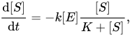
![{\displaystyle {\frac {{\text{d}}[S]}{{\text{d}}t}}=-k[E]{\frac {[S]}{K+[S]}},}](./_assets_/eb734a37dd21ce173a46342d1cc64c92/8b2328c322ac25f4e7b5538f71c094e3b93a75c3.svg) | | 4a |
![{\displaystyle {\frac {{\text{d}}[P]}{{\text{d}}t}}=-{\frac {{\text{d}}[S]}{{\text{d}}t}},}](./_assets_/eb734a37dd21ce173a46342d1cc64c92/0b0a0ac40d5ec30ce52ab24b94f7580fac37bb95.svg) | | 4b |
![{\displaystyle {\frac {{\text{d}}[B]}{{\text{d}}t}}=-Y{\frac {{\text{d}}[S]}{{\text{d}}t}}-\mu _{B}[B],}](./_assets_/eb734a37dd21ce173a46342d1cc64c92/44e4f6ccd6d4d304eebb6e0e56baf0c1657c0703.svg) | | 4c |
![{\displaystyle {\frac {{\text{d}}[E]}{{\text{d}}t}}=-zY{\frac {{\text{d}}[S]}{{\text{d}}t}}-\mu _{E}[E],}](./_assets_/eb734a37dd21ce173a46342d1cc64c92/530508be4e7f258dd84537cf94aade969bace46b.svg) | | 4d |
where
is the Michaelis–Menten constant (also known as the half-saturation concentration and affinity).
Implicit analytic solution
If one hypothesizes that the enzyme is produced at a rate proportional to the biomass production and degrades at a rate proportional to the biomass mortality, then Eqs. 4 can be rewritten as
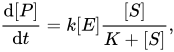
![{\displaystyle {\frac {{\text{d}}[P]}{{\text{d}}t}}=k[E]{\frac {[S]}{K+[S]}},}](./_assets_/eb734a37dd21ce173a46342d1cc64c92/de873d79f3d9ddce73d8e933e7e60ab50335a927.svg) | | 4a |
![{\displaystyle {\frac {{\text{d}}[S]}{{\text{d}}t}}=-{\frac {{\text{d}}[P]}{{\text{d}}t}},}](./_assets_/eb734a37dd21ce173a46342d1cc64c92/f04e7462200d809e93a97a65e9337505df32b73c.svg) | | 4b |
![{\displaystyle {\frac {{\text{d}}[B]}{{\text{d}}t}}=Y{\frac {{\text{d}}[P]}{{\text{d}}t}}-\mu _{B}[B],}](./_assets_/eb734a37dd21ce173a46342d1cc64c92/2961d9c3931b49da759e9320d0af8af447b70bff.svg) | | 4c |
![{\displaystyle {\frac {{\text{d}}[E]}{{\text{d}}t}}=-z{\frac {{\text{d}}[B]}{{\text{d}}t}},}](./_assets_/eb734a37dd21ce173a46342d1cc64c92/df8ecb07561e7507d18438057722c56562c4b061.svg) | | 4d |
where
,
,
,
are explicit function of time
. Note that Eq. (4b) and (4d) are linearly dependent on Eqs. (4a) and (4c), which are the two differential equations that can be used to solve the MMM problem. An implicit analytic solution[5] can be obtained if
is chosen as the independent variable and
,
,
and
) are rewritten as functions of
so to obtain

 | | 5a |
 | | 5b |
where
has been substituted by
as per mass balance
, with the initial value
when
, and where
has been substituted by
as per the linear relation
expressed by Eq. (4d). The analytic solution to Eq. (5b) is

 | | 6 |
with the initial biomass concentration
when
. To avoid the solution of a transcendental function, a polynomial Taylor expansion to the second-order in
is used for
in Eq. (6) as
 | | 7 |
Substituting Eq. (7) into Eq. (5a} and solving for
with the initial value
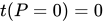
, one obtains the implicit solution for
as
 | | 8 |
with the constants
 | | 9a |

 | | 9b |
 | | 9c |
 | | 9d |
 | | 9e |
For any chosen value of
, the biomass concentration can be calculated with Eq. (7) at a time
given by Eq. (8). The corresponding values of
and
can be determined using the mass balances introduced above.