Mathematical description
Oseen looked for a solution for the Navier–Stokes equations in cylindrical coordinates  with velocity components
 of the form

where  is the circulation of the vortex core. Navier–Stokes equations lead to

which, subject to the conditions that it is regular at  and becomes unity as
 , leads to [3]

where  is the kinematic viscosity of the fluid. At
 , we have a potential vortex (free or irrotational vortex) with concentrated vorticity at the
 -axis; and this vorticity diffuses away as time passes.
The only non-zero vorticity component is in the -direction, given by

The pressure field simply ensures the vortex rotates in the circumferential direction, providing the centripetal force

where  is the constant density.[4] Below are two methods by which Oseen's vortex can be derived.
Derivation of the Lamb-Oseen vortex in polar coordinates
We begin with the polar coordinate  vector field,
 in which the azimuthal momentum equation reduces to the advectionless form,[3]
 which is subject to the following boundary conditions:
 By the substitution,
 , given some unknown
 , we have,
 We can invoke a self-similar solution,
 with
 , and obtain the following derivatives using the chain rule:
 By substitution, it follows that
 If
 , then
 , and hence,
 The first boundary condition,
 , infers that
 , which holds if and only if
 . Verifying by L'Hôpital's rule,
 The second boundary condition,
 , is satisfied by the irrotational vortex,
 , for all
 . Given the third boundary condition,
 , it follows that
 . Likewise,
 , the fourth boundary condition,
 , implies that
 , such that
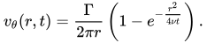
 . Therefore, the solution becomes
Alternative derivation of the Lamb-Oseen vortex by the vorticity equation
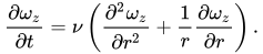
Given the vorticity vector,  , the -component of the linearized vorticity transport equation is [3]
 If one insists on invoking the similarity solution,
 with
 as done previously, one would exclusively obtain
 for arbitrary constants,
 and
 . To obtain the complete solution to
 , one must introduce the similarity solution,
 with
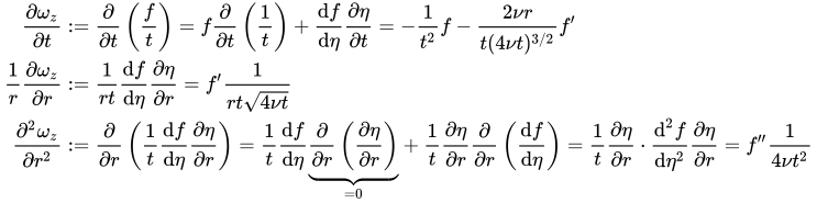
 . By the product rule and the chain rule, each derivative becomes,
 yielding the Sturm–Liouville differential equation,
 Because this is a differential equation of the form,
 for some function,
 , it admits the solution, [5]
 This can be checked by multiplying through by
 and using integration by parts as follows:
 Because
 is not well defined,
 . Substituting and
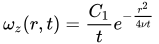
 into yields,
 The circulation flux integral over a surface,
 , may be solved for constant circulation, .[6]
:=\iint _{S}{\boldsymbol {\omega }}\cdot \mathrm {d} {\boldsymbol {S}}&=\int _{0}^{2\pi }\int _{0}^{\infty }\omega _{z}\cdot r\mathrm {d} r\mathrm {d} \theta \\&=2\pi \int _{0}^{\infty }{\frac {C_{1}}{t}}e^{-{\frac {r^{2}}{4\nu t}}}\cdot r\mathrm {d} r\\&=4\pi \nu C_{1}\int _{0}^{\infty }e^{-u}\mathrm {d} u\ \ \ {\text{where,}}\ \ \ u={\frac {r^{2}}{4\nu t}}\\\therefore C_{1}&={\frac {\Gamma }{4\pi \nu }}.\end{aligned}}}
 Since,
 bearing in mind that
 , we can use the integrating factor,
 , to isolate
 .
 The aforementioned boundary conditions on yields the Lamb-Oseen vortex.
Generalized Oseen vortex
The generalized Oseen vortex may be obtained by looking for solutions of the form

that leads to the equation

Self-similar solution exists for the coordinate , provided 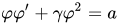 , where
 is a constant, in which case
 . The solution for
 may be written according to Rott (1958)[7] as

where  is an arbitrary constant. For
 , the classical Lamb–Oseen vortex is recovered. The case
 corresponds to the axisymmetric stagnation point flow, where
 is a constant. When
 ,
 , a Burgers vortex is a obtained. For arbitrary , the solution becomes
 , where
 is an arbitrary constant. As
 , Burgers vortex is recovered.

