Frobenius covariant

In matrix theory, the Frobenius covariants of a square matrix A are special polynomials of it, namely projection matrices F_i(A) associated with the eigenvalues and eigenvectors of A. They are named after the mathematician Ferdinand Frobenius.

Each covariant is a projection on the eigenspace associated with the eigenvalue λ_i. Frobenius covariants are the coefficients of Sylvester's formula, which expresses a function of a matrix f(A) as a matrix polynomial, namely a linear combination of that function's values on the eigenvalues of A.

Formal definition

Let A be a diagonalizable matrix with eigenvalues λ₁, ..., λ_k.

The Frobenius covariant F_i(A), for i = 1,..., k, is the matrix

$F_{i}(A)\equiv \prod _{j=1 \atop j\neq i}^{k}{\frac {1}{\lambda _{i}-\lambda _{j}}}(A-\lambda _{j}I)~.$

It is essentially the Lagrange polynomial with matrix argument. If the eigenvalue λ_i is simple, then as an idempotent projection matrix to a one-dimensional subspace, F_i(A) has a unit trace.

See also: Resolvent formalism

Computing the covariants

Ferdinand Georg Frobenius (1849–1917), German mathematician. His main interests were elliptic functions, differential equations, and later group theory.

The Frobenius covariants of a matrix A can be obtained from any eigendecomposition A = SDS⁻¹, where S is non-singular and D is diagonal with D_i,i = λ_i. The matrix S is defined up to multiplication on the right by a diagonal matrix. If A has no multiple eigenvalues, then let c_i be the ith right eigenvector of A, that is, the ith column of S; and let r_i be the ith left eigenvector of A, namely the ith row of S⁻¹. Then F_i(A) = c_i r_i. As a projection matrix, the Frobenius covariant satisfies the relation

$F_{i}(A)F_{j}(A)=\delta _{ij}F_{i}(A),$

which leads to r_i c_j = δ_ij.

Given that v and w are the right and left vectors satisfying w F_i(A) v ≠ 0, the right and left eigenvectors of A may be written as c_i = N_ci F_i(A) v and r_i = N_ri w F_i(A). The orthonormality of the eigenvectors gives one constraint for the normalization coefficients. The remaining freedom is related to the choice of representation for the matrix S.

If A has an eigenvalue λ_i appearing multiple times, then F_i(A) = Σ_j c_j r_j, where the sum is over all rows and columns associated with the eigenvalue λ_i.

Example

Consider the two-by-two matrix:

$A={\begin{bmatrix}1&3\\4&2\end{bmatrix}}.$

This matrix has two eigenvalues, 5 and −2, which can be found by solving the characteristic equation. By virtue of the Cayley–Hamilton theorem, (A − 5)(A + 2) = 0.

The corresponding eigen decomposition is

$A={\begin{bmatrix}3&1/7\\4&-1/7\end{bmatrix}}{\begin{bmatrix}5&0\\0&-2\end{bmatrix}}{\begin{bmatrix}3&1/7\\4&-1/7\end{bmatrix}}^{-1}={\begin{bmatrix}3&1/7\\4&-1/7\end{bmatrix}}{\begin{bmatrix}5&0\\0&-2\end{bmatrix}}{\begin{bmatrix}1/7&1/7\\4&-3\end{bmatrix}}.$

Hence the Frobenius covariants, manifestly projections, are

${\begin{array}{rl}F_{1}(A)&=c_{1}r_{1}={\begin{bmatrix}3\\4\end{bmatrix}}{\begin{bmatrix}1/7&1/7\end{bmatrix}}={\begin{bmatrix}3/7&3/7\\4/7&4/7\end{bmatrix}}=F_{1}^{2}(A)\\F_{2}(A)&=c_{2}r_{2}={\begin{bmatrix}1/7\\-1/7\end{bmatrix}}{\begin{bmatrix}4&-3\end{bmatrix}}={\begin{bmatrix}4/7&-3/7\\-4/7&3/7\end{bmatrix}}=F_{2}^{2}(A)~,\end{array}}$

with

$F_{1}(A)F_{2}(A)=0,\qquad F_{1}(A)+F_{2}(A)=I~.$

Note tr F₁(A) = tr F₂ (A)= 1, as required.

Generalization to defective matrices

Main article: Hermite interpolation § Explicit basis construction

When a square matrix ${\textstyle A\in \mathbb {C} ^{n\times n}}$ is defective (i.e., non-diagonalizable), its minimal polynomial contains repeated roots:

$$m(\lambda )=\prod _{i=1}^{k}(\lambda -\lambda _{i})^{m_{i}+1},$$

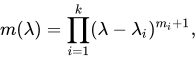
where ${\textstyle \lambda _{1},\dots ,\lambda _{k}}$ are the distinct eigenvalues of ${\textstyle A}$ with algebraic multiplicities ${\textstyle m_{i}+1}$ in the minimal polynomial.

Standard Frobenius covariants correspond to Lagrange interpolation, which applies only when all ${\textstyle m_{i}=0}$. For defective matrices, the definition generalizes via Hermite interpolation constructed through the Chinese remainder theorem.

Generalized Frobenius covariants

Using the CRT basis construction for Hermite interpolation, the basis scalar polynomials ${\textstyle f_{i,j}(\lambda )}$ for ${\textstyle 1\leq i\leq k}$ and ${\textstyle 0\leq j\leq m_{i}}$ are defined as:

$$f_{i,j}(\lambda )=f_{i}(\lambda )(\lambda -\lambda _{i})^{j}.$$

Here, the base polynomial is ${\textstyle f_{i}(\lambda )=u_{i}(\lambda )q_{i}(\lambda )}$, where ${\textstyle q_{i}(\lambda )=\prod _{r\neq i}(\lambda -\lambda _{r})^{m_{r}+1}}$. The polynomial ${\textstyle u_{i}(\lambda )}$ is computed using the extended Euclidean algorithm for polynomials to satisfy Bézout's identity:

$$u_{i}(\lambda )q_{i}(\lambda )+v_{i}(\lambda )(\lambda -\lambda _{i})^{m_{i}+1}=1.$$

Evaluating these basis polynomials at the matrix ${\textstyle A}$ yields the generalized Frobenius covariants ${\textstyle A_{i,j}\in \mathbb {C} ^{n\times n}}$:

$$A_{i,j}=f_{i,j}(A)=f_{i}(A)(A-\lambda _{i}I)^{j}.$$

The term ${\textstyle A_{i,0}=f_{i}(A)}$ represents the projection onto the generalized eigenspace corresponding to ${\textstyle \lambda _{i}}$, while ${\textstyle A_{i,j}}$ for ${\textstyle j>0}$ represents the associated nilpotent components (corresponding to the higher-order Jordan structure).

Matrix function evaluation

For any function ${\textstyle h(z)}$ that is sufficiently differentiable at each eigenvalue ${\textstyle \lambda _{i}}$ (up to order ${\textstyle m_{i}}$), the matrix function ${\textstyle h(A)}$ is given by the linear combination:

$$h(A)=\sum _{i=1}^{k}\sum _{j=0}^{m_{i}}{\frac {h^{(j)}(\lambda _{i})}{j!}}A_{i,j}.$$

In particular, setting ${\textstyle h(z)=z}$ provides the spectral decomposition (or Jordan–Chevalley decomposition) of ${\textstyle A}$ into its diagonalizable and nilpotent parts:

$$A=\sum _{i=1}^{k}\left(\lambda _{i}A_{i,0}+A_{i,1}\right).$$