Eigenvalue perturbation

Main article: Perturbation theory

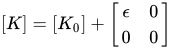
In mathematics, an eigenvalue perturbation problem is that of finding the eigenvectors and eigenvalues of a system $Ax=\lambda x$ that is perturbed from one with known eigenvectors and eigenvalues $A_{0}x_{0}=\lambda _{0}x_{0}$. This is useful for studying how sensitive the original system's eigenvectors and eigenvalues $x_{0i},\lambda _{0i},i=1,\dots n$ are to changes in the system. This type of analysis was popularized by Lord Rayleigh, in his investigation of harmonic vibrations of a string perturbed by small inhomogeneities.

The derivations in this article are essentially self-contained and can be found in many texts on numerical linear algebra or numerical functional analysis. This article is focused on the case of the perturbation of a simple eigenvalue, as opposed to a multiplicity of eigenvalues.

Motivation for generalized eigenvalues

Many scientific fields use eigenvalues to obtain solutions. Generalized eigenvalue problems are less widespread but are key in the study of vibrations. They are useful when the Galerkin or Rayleigh-Ritz methods are used to find approximate solutions of partial differential equations modeling vibrations of structures such as strings and plates - Courant (1943) is fundamental. The finite element method is a widespread particular case.

In classical mechanics, generalized eigenvalues may crop up when inspecting vibrations of multiple degrees of freedom systems close to equilibrium. In this case the kinetic energy provides the mass matrix $M$, the potential strain energy provides the rigidity matrix $K$.

With both methods, the following system of differential equations or matrix differential equation is derived: $M{\ddot {x}}+B{\dot {x}}+Kx=0$ with the mass matrix $M$ , the damping matrix $B$ and the rigidity matrix $K$. If the damping effect is neglected, $B=0$, and a solution of the form $x=e^{i\omega t}u$ is assumed,$u$ and $\omega ^{2}$are obtained as solutions to the generalized eigenvalue problem $-\omega ^{2}Mu+Ku=0$.

Setting of perturbation for a generalized eigenvalue problem

Suppose the solutions to the generalized eigenvalue problem are known to be

$\mathbf {K} _{0}\mathbf {x} _{0i}=\lambda _{0i}\mathbf {M} _{0}\mathbf {x} _{0i}.\qquad (0)$

where $\mathbf {K} _{0}$ and $\mathbf {M} _{0}$ are matrices. That is, we know the eigenvalues λ_0i and eigenvectors x_0i for i = 1, ..., N. An important note is that the eigenvalues are required to be distinct.

In order to perturb the matrices, one must find the eigenvalues and eigenvectors of

$\mathbf {K} \mathbf {x} _{i}=\lambda _{i}\mathbf {M} \mathbf {x} _{i}\qquad (1)$

where

${\begin{aligned}\mathbf {K} &=\mathbf {K} _{0}+\delta \mathbf {K} \\\mathbf {M} &=\mathbf {M} _{0}+\delta \mathbf {M} \end{aligned}}$

with the perturbations $\delta \mathbf {K}$ and $\delta \mathbf {M}$ much smaller than $\mathbf {K}$ and $\mathbf {M}$ respectively. Then the new eigenvalues and eigenvectors are expected to be similar to the original, plus small perturbations:

${\begin{aligned}\lambda _{i}&=\lambda _{0i}+\delta \lambda _{i}\\\mathbf {x} _{i}&=\mathbf {x} _{0i}+\delta \mathbf {x} _{i}\end{aligned}}$

Steps

Under the assumption that the matrices are symmetric, positive definite, and assume the eigenvectors are scaled such that

$\mathbf {x} _{0j}^{\top }\mathbf {M} _{0}\mathbf {x} _{0i}=\delta _{ij},\quad$$\mathbf {x} _{i}^{T}\mathbf {M} \mathbf {x} _{j}=\delta _{ij}\qquad (2)$

where δ_ij is the Kronecker delta. Now the equation to be solved is

$\mathbf {K} \mathbf {x} _{i}-\lambda _{i}\mathbf {M} \mathbf {x} _{i}=0.$

In this article, the study is restricted to first order perturbation.

First order expansion of the equation

Substituting in (1) results in

$(\mathbf {K} _{0}+\delta \mathbf {K} )(\mathbf {x} _{0i}+\delta \mathbf {x} _{i})=\left(\lambda _{0i}+\delta \lambda _{i}\right)\left(\mathbf {M} _{0}+\delta \mathbf {M} \right)\left(\mathbf {x} _{0i}+\delta \mathbf {x} _{i}\right),$

which expands to

${\begin{aligned}\mathbf {K} _{0}\mathbf {x} _{0i}&+\delta \mathbf {K} \mathbf {x} _{0i}+\mathbf {K} _{0}\delta \mathbf {x} _{i}+\delta \mathbf {K} \delta \mathbf {x} _{i}=\\[6pt]&\lambda _{0i}\mathbf {M} _{0}\mathbf {x} _{0i}+\lambda _{0i}\mathbf {M} _{0}\delta \mathbf {x} _{i}+\lambda _{0i}\delta \mathbf {M} \mathbf {x} _{0i}+\delta \lambda _{i}\mathbf {M} _{0}\mathbf {x} _{0i}+\\&\quad \lambda _{0i}\delta \mathbf {M} \delta \mathbf {x} _{i}+\delta \lambda _{i}\delta \mathbf {M} \mathbf {x} _{0i}+\delta \lambda _{i}\mathbf {M} _{0}\delta \mathbf {x} _{i}+\delta \lambda _{i}\delta \mathbf {M} \delta \mathbf {x} _{i}.\end{aligned}}$

Canceling from (0) ($\mathbf {K} _{0}\mathbf {x} _{0i}=\lambda _{0i}\mathbf {M} _{0}\mathbf {x} _{0i}$) leaves

${\begin{aligned}\delta \mathbf {K} \mathbf {x} _{0i}+&\mathbf {K} _{0}\delta \mathbf {x} _{i}+\delta \mathbf {K} \delta \mathbf {x} _{i}=\lambda _{0i}\mathbf {M} _{0}\delta \mathbf {x} _{i}+\lambda _{0i}\delta \mathbf {M} \mathbf {x} _{0i}+\delta \lambda _{i}\mathbf {M} _{0}\mathbf {x} _{0i}+\\&\lambda _{0i}\delta \mathbf {M} \delta \mathbf {x} _{i}+\delta \lambda _{i}\delta \mathbf {M} \mathbf {x} _{0i}+\delta \lambda _{i}\mathbf {M} _{0}\delta \mathbf {x} _{i}+\delta \lambda _{i}\delta \mathbf {M} \delta \mathbf {x} _{i}.\end{aligned}}$

Removing the higher-order terms, this simplifies to

$\mathbf {K} _{0}\delta \mathbf {x} _{i}+\delta \mathbf {K} \mathbf {x} _{0i}=\lambda _{0i}\mathbf {M} _{0}\delta \mathbf {x} _{i}+\lambda _{0i}\delta \mathbf {M} \mathrm {x} _{0i}+\delta \lambda _{i}\mathbf {M} _{0}\mathbf {x} _{0i}.\qquad (3)$

In other words, $\delta \lambda _{i}$ no longer denotes the exact variation of the eigenvalue but its first order approximation.

As the matrix is symmetric, the unperturbed eigenvectors are $M$ orthogonal and so can be used as a basis for the perturbed eigenvectors. This is the same as

$\delta \mathbf {x} _{i}=\sum _{j=1}^{N}\varepsilon _{ij}\mathbf {x} _{0j}\qquad (4)\quad$ with $\varepsilon _{ij}=\mathbf {x} _{0j}^{T}M\delta \mathbf {x} _{i}$,

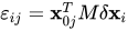where ε_ij are small constants that are to be determined.

In the same way, substituting in (2), and removing higher order terms, $\delta \mathbf {x} _{j}\mathbf {M} _{0}\mathbf {x} _{0i}+\mathbf {x} _{0j}\mathbf {M} _{0}\delta \mathbf {x} _{i}+\mathbf {x} _{0j}\delta \mathbf {M} _{0}\mathbf {x} _{0i}=0\quad {(5)}$

The derivation is then split into two paths.

First path: get first eigenvalue perturbation

Eigenvalue perturbation

Starting with (3)$\quad \mathbf {K} _{0}\delta \mathbf {x} _{i}+\delta \mathbf {K} \mathbf {x} _{0i}=\lambda _{0i}\mathbf {M} _{0}\delta \mathbf {x} _{i}+\lambda _{0i}\delta \mathbf {M} \mathrm {x} _{0i}+\delta \lambda _{i}\mathbf {M} _{0}\mathbf {x} _{0i};$which is then left multiplied with $\mathbf {x} _{0i}^{T}$ along with using (2) as well as its first order variation (5); one gets

$\mathbf {x} _{0i}^{T}\delta \mathbf {K} \mathbf {x} _{0i}=\lambda _{0i}\mathbf {x} _{0i}^{T}\delta \mathbf {M} \mathrm {x} _{0i}+\delta \lambda _{i}$

or

$\delta \lambda _{i}=\mathbf {x} _{0i}^{T}\delta \mathbf {K} \mathbf {x} _{0i}-\lambda _{0i}\mathbf {x} _{0i}^{T}\delta \mathbf {M} \mathrm {x} _{0i}$

This is the first order perturbation of the generalized Rayleigh quotient with fixed $x_{0i}$: $R(K,M;x_{0i})=x_{0i}^{T}Kx_{0i}/x_{0i}^{T}Mx_{0i},{\text{ with }}x_{0i}^{T}Mx_{0i}=1$

Moreover, for $M=I$, the formula $\delta \lambda _{i}=x_{0i}^{T}\delta Kx_{0i}$ should be compared with Bauer-Fike theorem which provides a bound for eigenvalue perturbation.

Eigenvector perturbation

One then left multiplies (3) with $x_{0j}^{T}$ for $j\neq i$ and get

$\mathbf {x} _{0j}^{T}\mathbf {K} _{0}\delta \mathbf {x} _{i}+\mathbf {x} _{0j}^{T}\delta \mathbf {K} \mathbf {x} _{0i}=\lambda _{0i}\mathbf {x} _{0j}^{T}\mathbf {M} _{0}\delta \mathbf {x} _{i}+\lambda _{0i}\mathbf {x} _{0j}^{T}\delta \mathbf {M} \mathrm {x} _{0i}+\delta \lambda _{i}\mathbf {x} _{0j}^{T}\mathbf {M} _{0}\mathbf {x} _{0i}.$

Recalling that $\mathbf {x} _{0j}^{T}K=\lambda _{0j}\mathbf {x} _{0j}^{T}M{\text{ and }}\mathbf {x} _{0j}^{T}\mathbf {M} _{0}\mathbf {x} _{0i}=0,$ for $j\neq i$, one may substitute for

$\lambda _{0j}\mathbf {x} _{0j}^{T}\mathbf {M} _{0}\delta \mathbf {x} _{i}+\mathbf {x} _{0j}^{T}\delta \mathbf {K} \mathbf {x} _{0i}=\lambda _{0i}\mathbf {x} _{0j}^{T}\mathbf {M} _{0}\delta \mathbf {x} _{i}+\lambda _{0i}\mathbf {x} _{0j}^{T}\delta \mathbf {M} \mathrm {x} _{0i}.$

or

$(\lambda _{0j}-\lambda _{0i})\mathbf {x} _{0j}^{T}\mathbf {M} _{0}\delta \mathbf {x} _{i}+\mathbf {x} _{0j}^{T}\delta \mathbf {K} \mathbf {x} _{0i}=\lambda _{0i}\mathbf {x} _{0j}^{T}\delta \mathbf {M} \mathrm {x} _{0i}.$

As the eigenvalues are assumed to be simple, for $j\neq i$

$\epsilon _{ij}=\mathbf {x} _{0j}^{T}\mathbf {M} _{0}\delta \mathbf {x} _{i}={\frac {-\mathbf {x} _{0j}^{T}\delta \mathbf {K} \mathbf {x} _{0i}+\lambda _{0i}\mathbf {x} _{0j}^{T}\delta \mathbf {M} \mathrm {x} _{0i}}{(\lambda _{0j}-\lambda _{0i})}},i=1,\dots N;j=1,\dots N;j\neq i.$

Moreover (5) (the first order variation of (2) ) yields $2\epsilon _{ii}=2\mathbf {x} _{0i}^{T}\mathbf {M} _{0}\delta x_{i}=-\mathbf {x} _{0i}^{T}\delta M\mathbf {x} _{0i}.$ All of the components of $\delta x_{i}$ have now been obtained.

Second path: Straightforward manipulations

Substituting (4) into (3) and rearranging gives

${\begin{aligned}\mathbf {K} _{0}\sum _{j=1}^{N}\varepsilon _{ij}\mathbf {x} _{0j}+\delta \mathbf {K} \mathbf {x} _{0i}&=\lambda _{0i}\mathbf {M} _{0}\sum _{j=1}^{N}\varepsilon _{ij}\mathbf {x} _{0j}+\lambda _{0i}\delta \mathbf {M} \mathbf {x} _{0i}+\delta \lambda _{i}\mathbf {M} _{0}\mathbf {x} _{0i}&&(5)\\\sum _{j=1}^{N}\varepsilon _{ij}\mathbf {K} _{0}\mathbf {x} _{0j}+\delta \mathbf {K} \mathbf {x} _{0i}&=\lambda _{0i}\mathbf {M} _{0}\sum _{j=1}^{N}\varepsilon _{ij}\mathbf {x} _{0j}+\lambda _{0i}\delta \mathbf {M} \mathbf {x} _{0i}+\delta \lambda _{i}\mathbf {M} _{0}\mathbf {x} _{0i}&&\\({\text{applying }}\mathbf {K} _{0}{\text{ to the sum}})\\\sum _{j=1}^{N}\varepsilon _{ij}\lambda _{0j}\mathbf {M} _{0}\mathbf {x} _{0j}+\delta \mathbf {K} \mathbf {x} _{0i}&=\lambda _{0i}\mathbf {M} _{0}\sum _{j=1}^{N}\varepsilon _{ij}\mathbf {x} _{0j}+\lambda _{0i}\delta \mathbf {M} \mathbf {x} _{0i}+\delta \lambda _{i}\mathbf {M} _{0}\mathbf {x} _{0i}&&({\text{using Eq. }}(1))\end{aligned}}$

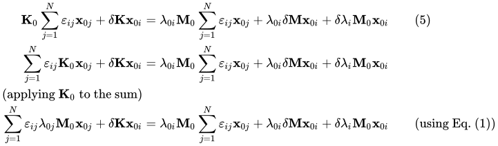
Because the eigenvectors are M₀-orthogonal when M₀ is positive definite, one can remove the summations by left-multiplying by $\mathbf {x} _{0i}^{\top }$:

$\mathbf {x} _{0i}^{\top }\varepsilon _{ii}\lambda _{0i}\mathbf {M} _{0}\mathbf {x} _{0i}+\mathbf {x} _{0i}^{\top }\delta \mathbf {K} \mathbf {x} _{0i}=\lambda _{0i}\mathbf {x} _{0i}^{\top }\mathbf {M} _{0}\varepsilon _{ii}\mathbf {x} _{0i}+\lambda _{0i}\mathbf {x} _{0i}^{\top }\delta \mathbf {M} \mathbf {x} _{0i}+\delta \lambda _{i}\mathbf {x} _{0i}^{\top }\mathbf {M} _{0}\mathbf {x} _{0i}.$

By use of equation (1) again:

$\mathbf {x} _{0i}^{\top }\mathbf {K} _{0}\varepsilon _{ii}\mathbf {x} _{0i}+\mathbf {x} _{0i}^{\top }\delta \mathbf {K} \mathbf {x} _{0i}=\lambda _{0i}\mathbf {x} _{0i}^{\top }\mathbf {M} _{0}\varepsilon _{ii}\mathbf {x} _{0i}+\lambda _{0i}\mathbf {x} _{0i}^{\top }\delta \mathbf {M} \mathbf {x} _{0i}+\delta \lambda _{i}\mathbf {x} _{0i}^{\top }\mathbf {M} _{0}\mathbf {x} _{0i}.\qquad (6)$

The two terms containing ε_ii are equal because left-multiplying (1) by $\mathbf {x} _{0i}^{\top }$ gives

$\mathbf {x} _{0i}^{\top }\mathbf {K} _{0}\mathbf {x} _{0i}=\lambda _{0i}\mathbf {x} _{0i}^{\top }\mathbf {M} _{0}\mathbf {x} _{0i}.$

Canceling those terms in (6) leaves

$\mathbf {x} _{0i}^{\top }\delta \mathbf {K} \mathbf {x} _{0i}=\lambda _{0i}\mathbf {x} _{0i}^{\top }\delta \mathbf {M} \mathbf {x} _{0i}+\delta \lambda _{i}\mathbf {x} _{0i}^{\top }\mathbf {M} _{0}\mathbf {x} _{0i}.$

Rearranging gives

$\delta \lambda _{i}={\frac {\mathbf {x} _{0i}^{\top }\left(\delta \mathbf {K} -\lambda _{0i}\delta \mathbf {M} \right)\mathbf {x} _{0i}}{\mathbf {x} _{0i}^{\top }\mathbf {M} _{0}\mathbf {x} _{0i}}}$

But by (2), this denominator is equal to 1. Thus

$\delta \lambda _{i}=\mathbf {x} _{0i}^{\top }\left(\delta \mathbf {K} -\lambda _{0i}\delta \mathbf {M} \right)\mathbf {x} _{0i}.$

Then, as $\lambda _{i}\neq \lambda _{k}$ for $i\neq k$ (this is the assumption of simple eigenvalues) by left-multiplying equation (5) by $\mathbf {x} _{0k}^{\top }$:

$\varepsilon _{ik}={\frac {\mathbf {x} _{0k}^{\top }\left(\delta \mathbf {K} -\lambda _{0i}\delta \mathbf {M} \right)\mathbf {x} _{0i}}{\lambda _{0i}-\lambda _{0k}}},\qquad i\neq k.$

Or by changing the name of the indices:

$\varepsilon _{ij}={\frac {\mathbf {x} _{0j}^{\top }\left(\delta \mathbf {K} -\lambda _{0i}\delta \mathbf {M} \right)\mathbf {x} _{0i}}{\lambda _{0i}-\lambda _{0j}}},\qquad i\neq j.$

To find ε_ii, using the fact that

$\mathbf {x} _{i}^{\top }\mathbf {M} \mathbf {x} _{i}=1$

implies:

$\varepsilon _{ii}=-{\tfrac {1}{2}}\mathbf {x} _{0i}^{\top }\delta \mathbf {M} \mathbf {x} _{0i}.$

Summary of the first order perturbation result

In the case where all the matrices are Hermitian positive definite and all the eigenvalues are distinct,

${\begin{aligned}\lambda _{i}&=\lambda _{0i}+\mathbf {x} _{0i}^{\top }\left(\delta \mathbf {K} -\lambda _{0i}\delta \mathbf {M} \right)\mathbf {x} _{0i}\\\mathbf {x} _{i}&=\mathbf {x} _{0i}\left(1-{\tfrac {1}{2}}\mathbf {x} _{0i}^{\top }\delta \mathbf {M} \mathbf {x} _{0i}\right)+\sum _{j=1 \atop j\neq i}^{N}{\frac {\mathbf {x} _{0j}^{\top }\left(\delta \mathbf {K} -\lambda _{0i}\delta \mathbf {M} \right)\mathbf {x} _{0i}}{\lambda _{0i}-\lambda _{0j}}}\mathbf {x} _{0j}\end{aligned}}$

for infinitesimal $\delta \mathbf {K}$ and $\delta \mathbf {M}$ (the higher order terms in (3) being neglected).

A proof that higher order terms may be neglect may be derived using the implicit function theorem.

Theoretical derivation

Perturbation of an implicit function.

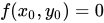In the next paragraph, we shall use the Implicit function theorem (Statement of the theorem ); we notice that for a continuously differentiable function $f:\mathbb {R} ^{n+m}\to \mathbb {R} ^{m},\;f:(x,y)\mapsto f(x,y)$, with an invertible Jacobian matrix $J_{f,b}(x_{0},y_{0})$, from a point $(x_{0},y_{0})$ solution of $f(x_{0},y_{0})=0$, we get solutions of $f(x,y)=0$ with $x$ close to $x_{0}$ in the form $y=g(x)$ where $g$ is a continuously differentiable function ; moreover the Jacobian marix of $g$ is provided by the linear system

$J_{f,y}(x,g(x))J_{g,x}(x)+J_{f,x}(x,g(x))=0\quad (6)$.

As soon as the hypothesis of the theorem is satisfied, the Jacobian matrix of $g$ may be computed with a first order expansion of $f(x_{0}+\delta x,y_{0}+\delta y)=0$, we get

$J_{f,x}(x,g(x))\delta x+J_{f,y}(x,g(x))\delta y=0$; as $\delta y=J_{g,x}(x)\delta x$, it is equivalent to equation $(6)$.

Eigenvalue perturbation: a theoretical basis.

We use the previous paragraph (Perturbation of an implicit function) with somewhat different notations suited to eigenvalue perturbation; we introduce ${\tilde {f}}:\mathbb {R} ^{2n^{2}}\times \mathbb {R} ^{n+1}\to \mathbb {R} ^{n+1}$, with

• ${\tilde {f}}(K,M,\lambda ,x)={\binom {f(K,M,\lambda ,x)}{f_{n+1}(x)}}$ with

$f(K,M,\lambda ,x)=Kx-\lambda x,f_{n+1}(M,x)=x^{T}Mx-1$. In order to use the Implicit function theorem, we study the invertibility of the Jacobian $J_{{\tilde {f}};\lambda ,x}(K,M;\lambda _{0i},x_{0i})$ with

$J_{{\tilde {f}};\lambda ,x}(K,M;\lambda _{i},x_{i})(\delta \lambda ,\delta x)={\binom {-Mx_{i}}{0}}\delta \lambda +{\binom {K-\lambda M}{2x_{i}^{T}M}}\delta x_{i}$. Indeed, the solution of

$J_{{\tilde {f}};\lambda _{0i},x_{0i}}(K,M;\lambda _{0i},x_{0i})(\delta \lambda _{i},\delta x_{i})=$${\binom {y}{y_{n+1}}}$ may be derived with computations similar to the derivation of the expansion.

$$\delta \lambda _{i}=-x_{0i}^{T}y,\;{\text{ and }}(\lambda _{0i}-\lambda _{0j})x_{0j}^{T}M\delta x_{i}=x_{j}^{T}y,j=1,\dots ,n,j\neq i\;;$$ ${\text{ or }}x_{0j}^{T}M\delta x_{i}=x_{j}^{T}y/(\lambda _{0i}-\lambda _{0j}),{\text{ and }}\;2x_{0i}^{T}M\delta x_{i}=y_{n+1}$

When $\lambda _{i}$ is a simple eigenvalue, as the eigenvectors $x_{0j},j=1,\dots ,n$ form an orthonormal basis, for any right-hand side, we have obtained one solution therefore, the Jacobian is invertible.

The implicit function theorem provides a continuously differentiable function $(K,M)\mapsto (\lambda _{i}(K,M),x_{i}(K,M))$ hence the expansion with little o notation: $\lambda _{i}=\lambda _{0i}+\delta \lambda _{i}+o(\|\delta K\|+\|\delta M\|)$ $x_{i}=x_{0i}+\delta x_{i}+o(\|\delta K\|+\|\delta M\|)$. with

$\delta \lambda _{i}=\mathbf {x} _{0i}^{T}\delta \mathbf {K} \mathbf {x} _{0i}-\lambda _{0i}\mathbf {x} _{0i}^{T}\delta \mathbf {M} \mathrm {x} _{0i};$ $\delta x_{i}=\mathbf {x} _{0j}^{T}\mathbf {M} _{0}\delta \mathbf {x} _{i}\mathbf {x} _{0j}{\text{ with}}$$\mathbf {x} _{0j}^{T}\mathbf {M} _{0}\delta \mathbf {x} _{i}={\frac {-\mathbf {x} _{0j}^{T}\delta \mathbf {K} \mathbf {x} _{0i}+\lambda _{0i}\mathbf {x} _{0j}^{T}\delta \mathbf {M} \mathrm {x} _{0i}}{(\lambda _{0j}-\lambda _{0i})}},i=1,\dots n;j=1,\dots n;j\neq i.$ This is the first order expansion of the perturbed eigenvalues and eigenvectors. which is proved.

Results of sensitivity analysis with respect to the entries of the matrices

The results

This means it is possible to efficiently do a sensitivity analysis on λ_i as a function of changes in the entries of the matrices. (Recall that the matrices are symmetric and so changing K_kℓ will also change K_ℓk, hence the (2 − δ_kℓ) term

Why generalized eigenvalues?

In the entry applications of eigenvalues and eigenvectors we find numerous scientific fields in which eigenvalues are used to obtain solutions. Generalized eigenvalue problems are less widespread but are a key in the study of vibrations. They are useful when we use the Galerkin method or Rayleigh-Ritz method to find approximate solutions of partial differential equations modeling vibrations of structures such as strings and plates; the paper of Courant (1943) is fundamental. The Finite element method is a widespread particular case.

In classical mechanics, generalized eigenvalues may crop up when we look for vibrations of multiple degrees of freedom systems close to equilibrium; the kinetic energy provides the mass matrix $M$, the potential strain energy provides the rigidity matrix $K$. For further details, see the first section of this article of Weinstein (1941, in French)

With both methods, we obtain a system of differential equations or Matrix differential equation $M{\ddot {x}}+B{\dot {x}}+Kx=0$ with the mass matrix $M$ , the damping matrix $B$ and the rigidity matrix $K$. If we neglect the damping effect, we use $B=0$, we can look for a solution of the following form $x=e^{i\omega t}u$; we obtain that $u$ and $\omega ^{2}$are solution of the generalized eigenvalue problem $-\omega ^{2}Mu+Ku=0$

Setting of perturbation for a generalized eigenvalue problem

Suppose we have solutions to the generalized eigenvalue problem,

$\mathbf {K} _{0}\mathbf {x} _{0i}=\lambda _{0i}\mathbf {M} _{0}\mathbf {x} _{0i}.\qquad (0)$

where $\mathbf {K} _{0}$ and $\mathbf {M} _{0}$ are matrices. That is, we know the eigenvalues λ_0i and eigenvectors x_0i for i = 1, ..., N. It is also required that the eigenvalues are distinct.

Now suppose we want to change the matrices by a small amount. That is, we want to find the eigenvalues and eigenvectors of

$\mathbf {K} \mathbf {x} _{i}=\lambda _{i}\mathbf {M} \mathbf {x} _{i}\qquad (1)$

where

${\begin{aligned}\mathbf {K} &=\mathbf {K} _{0}+\delta \mathbf {K} \\\mathbf {M} &=\mathbf {M} _{0}+\delta \mathbf {M} \end{aligned}}$

with the perturbations $\delta \mathbf {K}$ and $\delta \mathbf {M}$ much smaller than $\mathbf {K}$ and $\mathbf {M}$ respectively. Then we expect the new eigenvalues and eigenvectors to be similar to the original, plus small perturbations:

${\begin{aligned}\lambda _{i}&=\lambda _{0i}+\delta \lambda _{i}\\\mathbf {x} _{i}&=\mathbf {x} _{0i}+\delta \mathbf {x} _{i}\end{aligned}}$

Steps

We assume that the matrices are symmetric and positive definite, and assume we have scaled the eigenvectors such that

$\mathbf {x} _{0j}^{\top }\mathbf {M} _{0}\mathbf {x} _{0i}=\delta _{ij},\quad$$\mathbf {x} _{i}^{T}\mathbf {M} \mathbf {x} _{j}=\delta _{ij}\qquad (2)$

where δ_ij is the Kronecker delta. Now we want to solve the equation

$\mathbf {K} \mathbf {x} _{i}-\lambda _{i}\mathbf {M} \mathbf {x} _{i}=0.$

In this article we restrict the study to first order perturbation.

First order expansion of the equation

Substituting in (1), we get

$(\mathbf {K} _{0}+\delta \mathbf {K} )(\mathbf {x} _{0i}+\delta \mathbf {x} _{i})=\left(\lambda _{0i}+\delta \lambda _{i}\right)\left(\mathbf {M} _{0}+\delta \mathbf {M} \right)\left(\mathbf {x} _{0i}+\delta \mathbf {x} _{i}\right),$

which expands to

${\begin{aligned}\mathbf {K} _{0}\mathbf {x} _{0i}&+\delta \mathbf {K} \mathbf {x} _{0i}+\mathbf {K} _{0}\delta \mathbf {x} _{i}+\delta \mathbf {K} \delta \mathbf {x} _{i}=\\[6pt]&\lambda _{0i}\mathbf {M} _{0}\mathbf {x} _{0i}+\lambda _{0i}\mathbf {M} _{0}\delta \mathbf {x} _{i}+\lambda _{0i}\delta \mathbf {M} \mathbf {x} _{0i}+\delta \lambda _{i}\mathbf {M} _{0}\mathbf {x} _{0i}+\\&\quad \lambda _{0i}\delta \mathbf {M} \delta \mathbf {x} _{i}+\delta \lambda _{i}\delta \mathbf {M} \mathbf {x} _{0i}+\delta \lambda _{i}\mathbf {M} _{0}\delta \mathbf {x} _{i}+\delta \lambda _{i}\delta \mathbf {M} \delta \mathbf {x} _{i}.\end{aligned}}$

Canceling from (0) ($\mathbf {K} _{0}\mathbf {x} _{0i}=\lambda _{0i}\mathbf {M} _{0}\mathbf {x} _{0i}$) leaves

${\begin{aligned}\delta \mathbf {K} \mathbf {x} _{0i}+&\mathbf {K} _{0}\delta \mathbf {x} _{i}+\delta \mathbf {K} \delta \mathbf {x} _{i}=\lambda _{0i}\mathbf {M} _{0}\delta \mathbf {x} _{i}+\lambda _{0i}\delta \mathbf {M} \mathbf {x} _{0i}+\delta \lambda _{i}\mathbf {M} _{0}\mathbf {x} _{0i}+\\&\lambda _{0i}\delta \mathbf {M} \delta \mathbf {x} _{i}+\delta \lambda _{i}\delta \mathbf {M} \mathbf {x} _{0i}+\delta \lambda _{i}\mathbf {M} _{0}\delta \mathbf {x} _{i}+\delta \lambda _{i}\delta \mathbf {M} \delta \mathbf {x} _{i}.\end{aligned}}$

Removing the higher-order terms, this simplifies to

$\mathbf {K} _{0}\delta \mathbf {x} _{i}+\delta \mathbf {K} \mathbf {x} _{0i}=\lambda _{0i}\mathbf {M} _{0}\delta \mathbf {x} _{i}+\lambda _{0i}\delta \mathbf {M} \mathrm {x} _{0i}+\delta \lambda _{i}\mathbf {M} _{0}\mathbf {x} _{0i}.\qquad (3)$

In other words, $\delta \lambda _{i}$ no longer denotes the exact variation of the eigenvalue but its first order approximation.

As the matrix is symmetric, the unperturbed eigenvectors are $M$ orthogonal and so we use them as a basis for the perturbed eigenvectors. That is, we want to construct

$\delta \mathbf {x} _{i}=\sum _{j=1}^{N}\varepsilon _{ij}\mathbf {x} _{0j}\qquad (4)\quad$ with $\varepsilon _{ij}=\mathbf {x} _{0j}^{T}M\delta \mathbf {x} _{i}$,

where the ε_ij are small constants that are to be determined.

In the same way, substituting in (2), and removing higher order terms, we get $\delta \mathbf {x} _{j}\mathbf {M} _{0}\mathbf {x} _{0i}+\mathbf {x} _{0j}\mathbf {M} _{0}\delta \mathbf {x} _{i}+\mathbf {x} _{0j}\delta \mathbf {M} _{0}\mathbf {x} _{0i}=0\quad {(5)}$

The derivation can go on with two forks.

First fork: get first eigenvalue perturbation

Eigenvalue perturbation

We start with (3)$\quad \mathbf {K} _{0}\delta \mathbf {x} _{i}+\delta \mathbf {K} \mathbf {x} _{0i}=\lambda _{0i}\mathbf {M} _{0}\delta \mathbf {x} _{i}+\lambda _{0i}\delta \mathbf {M} \mathrm {x} _{0i}+\delta \lambda _{i}\mathbf {M} _{0}\mathbf {x} _{0i};$

we left multiply with $\mathbf {x} _{0i}^{T}$ and use (2) as well as its first order variation (5); we get

$\mathbf {x} _{0i}^{T}\delta \mathbf {K} \mathbf {x} _{0i}=\lambda _{0i}\mathbf {x} _{0i}^{T}\delta \mathbf {M} \mathrm {x} _{0i}+\delta \lambda _{i}$

or

$\delta \lambda _{i}=\mathbf {x} _{0i}^{T}\delta \mathbf {K} \mathbf {x} _{0i}-\lambda _{0i}\mathbf {x} _{0i}^{T}\delta \mathbf {M} \mathrm {x} _{0i}$

We notice that it is the first order perturbation of the generalized Rayleigh quotient with fixed $x_{0i}$: $R(K,M;x_{0i})=x_{0i}^{T}Kx_{0i}/x_{0i}^{T}Mx_{0i},{\text{ with }}x_{0i}^{T}Mx_{0i}=1$

Moreover, for $M=I$, the formula $\delta \lambda _{i}=x_{0i}^{T}\delta Kx_{0i}$ should be compared with Bauer-Fike theorem which provides a bound for eigenvalue perturbation.

Eigenvector perturbation

We left multiply (3) with $x_{0j}^{T}$ for $j\neq i$ and get

$\mathbf {x} _{0j}^{T}\mathbf {K} _{0}\delta \mathbf {x} _{i}+\mathbf {x} _{0j}^{T}\delta \mathbf {K} \mathbf {x} _{0i}=\lambda _{0i}\mathbf {x} _{0j}^{T}\mathbf {M} _{0}\delta \mathbf {x} _{i}+\lambda _{0i}\mathbf {x} _{0j}^{T}\delta \mathbf {M} \mathrm {x} _{0i}+\delta \lambda _{i}\mathbf {x} _{0j}^{T}\mathbf {M} _{0}\mathbf {x} _{0i}.$

We use $\mathbf {x} _{0j}^{T}K=\lambda _{0j}\mathbf {x} _{0j}^{T}M{\text{ and }}\mathbf {x} _{0j}^{T}\mathbf {M} _{0}\mathbf {x} _{0i}=0,$ for $j\neq i$.

$\lambda _{0j}\mathbf {x} _{0j}^{T}\mathbf {M} _{0}\delta \mathbf {x} _{i}+\mathbf {x} _{0j}^{T}\delta \mathbf {K} \mathbf {x} _{0i}=\lambda _{0i}\mathbf {x} _{0j}^{T}\mathbf {M} _{0}\delta \mathbf {x} _{i}+\lambda _{0i}\mathbf {x} _{0j}^{T}\delta \mathbf {M} \mathrm {x} _{0i}.$

or

$(\lambda _{0j}-\lambda _{0i})\mathbf {x} _{0j}^{T}\mathbf {M} _{0}\delta \mathbf {x} _{i}+\mathbf {x} _{0j}^{T}\delta \mathbf {K} \mathbf {x} _{0i}=\lambda _{0i}\mathbf {x} _{0j}^{T}\delta \mathbf {M} \mathrm {x} _{0i}.$

As the eigenvalues are assumed to be simple, for $j\neq i$

$\epsilon _{ij}=\mathbf {x} _{0j}^{T}\mathbf {M} _{0}\delta \mathbf {x} _{i}={\frac {-\mathbf {x} _{0j}^{T}\delta \mathbf {K} \mathbf {x} _{0i}+\lambda _{0i}\mathbf {x} _{0j}^{T}\delta \mathbf {M} \mathrm {x} _{0i}}{(\lambda _{0j}-\lambda _{0i})}},i=1,\dots N;j=1,\dots N;j\neq i.$

Moreover (5) (the first order variation of (2) ) yields $2\epsilon _{ii}=2\mathbf {x} _{0i}^{T}\mathbf {M} _{0}\delta x_{i}=-\mathbf {x} _{0i}^{T}\delta M\mathbf {x} _{0i}.$ We have obtained all the components of $\delta x_{i}$ .

Second fork: Straightforward manipulations

Substituting (4) into (3) and rearranging gives

${\begin{aligned}\mathbf {K} _{0}\sum _{j=1}^{N}\varepsilon _{ij}\mathbf {x} _{0j}+\delta \mathbf {K} \mathbf {x} _{0i}&=\lambda _{0i}\mathbf {M} _{0}\sum _{j=1}^{N}\varepsilon _{ij}\mathbf {x} _{0j}+\lambda _{0i}\delta \mathbf {M} \mathbf {x} _{0i}+\delta \lambda _{i}\mathbf {M} _{0}\mathbf {x} _{0i}&&(5)\\\sum _{j=1}^{N}\varepsilon _{ij}\mathbf {K} _{0}\mathbf {x} _{0j}+\delta \mathbf {K} \mathbf {x} _{0i}&=\lambda _{0i}\mathbf {M} _{0}\sum _{j=1}^{N}\varepsilon _{ij}\mathbf {x} _{0j}+\lambda _{0i}\delta \mathbf {M} \mathbf {x} _{0i}+\delta \lambda _{i}\mathbf {M} _{0}\mathbf {x} _{0i}&&\\({\text{applying }}\mathbf {K} _{0}{\text{ to the sum}})\\\sum _{j=1}^{N}\varepsilon _{ij}\lambda _{0j}\mathbf {M} _{0}\mathbf {x} _{0j}+\delta \mathbf {K} \mathbf {x} _{0i}&=\lambda _{0i}\mathbf {M} _{0}\sum _{j=1}^{N}\varepsilon _{ij}\mathbf {x} _{0j}+\lambda _{0i}\delta \mathbf {M} \mathbf {x} _{0i}+\delta \lambda _{i}\mathbf {M} _{0}\mathbf {x} _{0i}&&({\text{using Eq. }}(1))\end{aligned}}$

Because the eigenvectors are M₀-orthogonal when M₀ is positive definite, we can remove the summations by left-multiplying by $\mathbf {x} _{0i}^{\top }$:

$\mathbf {x} _{0i}^{\top }\varepsilon _{ii}\lambda _{0i}\mathbf {M} _{0}\mathbf {x} _{0i}+\mathbf {x} _{0i}^{\top }\delta \mathbf {K} \mathbf {x} _{0i}=\lambda _{0i}\mathbf {x} _{0i}^{\top }\mathbf {M} _{0}\varepsilon _{ii}\mathbf {x} _{0i}+\lambda _{0i}\mathbf {x} _{0i}^{\top }\delta \mathbf {M} \mathbf {x} _{0i}+\delta \lambda _{i}\mathbf {x} _{0i}^{\top }\mathbf {M} _{0}\mathbf {x} _{0i}.$

By use of equation (1) again:

$\mathbf {x} _{0i}^{\top }\mathbf {K} _{0}\varepsilon _{ii}\mathbf {x} _{0i}+\mathbf {x} _{0i}^{\top }\delta \mathbf {K} \mathbf {x} _{0i}=\lambda _{0i}\mathbf {x} _{0i}^{\top }\mathbf {M} _{0}\varepsilon _{ii}\mathbf {x} _{0i}+\lambda _{0i}\mathbf {x} _{0i}^{\top }\delta \mathbf {M} \mathbf {x} _{0i}+\delta \lambda _{i}\mathbf {x} _{0i}^{\top }\mathbf {M} _{0}\mathbf {x} _{0i}.\qquad (6)$

The two terms containing ε_ii are equal because left-multiplying (1) by $\mathbf {x} _{0i}^{\top }$ gives

$\mathbf {x} _{0i}^{\top }\mathbf {K} _{0}\mathbf {x} _{0i}=\lambda _{0i}\mathbf {x} _{0i}^{\top }\mathbf {M} _{0}\mathbf {x} _{0i}.$

Canceling those terms in (6) leaves

$\mathbf {x} _{0i}^{\top }\delta \mathbf {K} \mathbf {x} _{0i}=\lambda _{0i}\mathbf {x} _{0i}^{\top }\delta \mathbf {M} \mathbf {x} _{0i}+\delta \lambda _{i}\mathbf {x} _{0i}^{\top }\mathbf {M} _{0}\mathbf {x} _{0i}.$

Rearranging gives

$\delta \lambda _{i}={\frac {\mathbf {x} _{0i}^{\top }\left(\delta \mathbf {K} -\lambda _{0i}\delta \mathbf {M} \right)\mathbf {x} _{0i}}{\mathbf {x} _{0i}^{\top }\mathbf {M} _{0}\mathbf {x} _{0i}}}$

But by (2), this denominator is equal to 1. Thus

$\delta \lambda _{i}=\mathbf {x} _{0i}^{\top }\left(\delta \mathbf {K} -\lambda _{0i}\delta \mathbf {M} \right)\mathbf {x} _{0i}.$

Then, as $\lambda _{i}\neq \lambda _{k}$ for $i\neq k$ (assumption simple eigenvalues) by left-multiplying equation (5) by $\mathbf {x} _{0k}^{\top }$:

$\varepsilon _{ik}={\frac {\mathbf {x} _{0k}^{\top }\left(\delta \mathbf {K} -\lambda _{0i}\delta \mathbf {M} \right)\mathbf {x} _{0i}}{\lambda _{0i}-\lambda _{0k}}},\qquad i\neq k.$

Or by changing the name of the indices:

$\varepsilon _{ij}={\frac {\mathbf {x} _{0j}^{\top }\left(\delta \mathbf {K} -\lambda _{0i}\delta \mathbf {M} \right)\mathbf {x} _{0i}}{\lambda _{0i}-\lambda _{0j}}},\qquad i\neq j.$

To find ε_ii, use the fact that:

$\mathbf {x} _{i}^{\top }\mathbf {M} \mathbf {x} _{i}=1$

implies:

$\varepsilon _{ii}=-{\tfrac {1}{2}}\mathbf {x} _{0i}^{\top }\delta \mathbf {M} \mathbf {x} _{0i}.$

Summary of the first order perturbation result

In the case where all the matrices are Hermitian positive definite and all the eigenvalues are distinct,

${\begin{aligned}\lambda _{i}&=\lambda _{0i}+\mathbf {x} _{0i}^{\top }\left(\delta \mathbf {K} -\lambda _{0i}\delta \mathbf {M} \right)\mathbf {x} _{0i}\\\mathbf {x} _{i}&=\mathbf {x} _{0i}\left(1-{\tfrac {1}{2}}\mathbf {x} _{0i}^{\top }\delta \mathbf {M} \mathbf {x} _{0i}\right)+\sum _{j=1 \atop j\neq i}^{N}{\frac {\mathbf {x} _{0j}^{\top }\left(\delta \mathbf {K} -\lambda _{0i}\delta \mathbf {M} \right)\mathbf {x} _{0i}}{\lambda _{0i}-\lambda _{0j}}}\mathbf {x} _{0j}\end{aligned}}$

for infinitesimal $\delta \mathbf {K}$ and $\delta \mathbf {M}$ (the higher order terms in (3) being neglected).

So far, we have not proved that these higher order terms may be neglected. This point may be derived using the implicit function theorem; in next section, we summarize the use of this theorem in order to obtain a first order expansion.

Theoretical derivation

Perturbation of an implicit function.

In the next paragraph, we shall use the Implicit function theorem (Statement of the theorem ); we notice that for a continuously differentiable function $f:\mathbb {R} ^{n+m}\to \mathbb {R} ^{m},\;f:(x,y)\mapsto f(x,y)$, with an invertible Jacobian matrix $J_{f,b}(x_{0},y_{0})$, from a point $(x_{0},y_{0})$ solution of $f(x_{0},y_{0})=0$, we get solutions of $f(x,y)=0$ with $x$ close to $x_{0}$ in the form $y=g(x)$ where $g$ is a continuously differentiable function ; moreover the Jacobian marix of $g$ is provided by the linear system

$J_{f,y}(x,g(x))J_{g,x}(x)+J_{f,x}(x,g(x))=0\quad (6)$.

As soon as the hypothesis of the theorem is satisfied, the Jacobian matrix of $g$ may be computed with a first order expansion of $f(x_{0}+\delta x,y_{0}+\delta y)=0$, we get

$J_{f,x}(x,g(x))\delta x+J_{f,y}(x,g(x))\delta y=0$; as $\delta y=J_{g,x}(x)\delta x$, it is equivalent to equation $(6)$.

Eigenvalue perturbation: a theoretical basis.

We use the previous paragraph (Perturbation of an implicit function) with somewhat different notations suited to eigenvalue perturbation; we introduce ${\tilde {f}}:\mathbb {R} ^{2n^{2}}\times \mathbb {R} ^{n+1}\to \mathbb {R} ^{n+1}$, with

• ${\tilde {f}}(K,M,\lambda ,x)={\binom {f(K,M,\lambda ,x)}{f_{n+1}(x)}}$ with

$f(K,M,\lambda ,x)=Kx-\lambda x,f_{n+1}(M,x)=x^{T}Mx-1$. In order to use the Implicit function theorem, we study the invertibility of the Jacobian $J_{{\tilde {f}};\lambda ,x}(K,M;\lambda _{0i},x_{0i})$ with

$J_{{\tilde {f}};\lambda ,x}(K,M;\lambda _{i},x_{i})(\delta \lambda ,\delta x)={\binom {-Mx_{i}}{0}}\delta \lambda +{\binom {K-\lambda M}{2x_{i}^{T}M}}\delta x_{i}$. Indeed, the solution of

$J_{{\tilde {f}};\lambda _{0i},x_{0i}}(K,M;\lambda _{0i},x_{0i})(\delta \lambda _{i},\delta x_{i})=$${\binom {y}{y_{n+1}}}$ may be derived with computations similar to the derivation of the expansion.

$$\delta \lambda _{i}=-x_{0i}^{T}y,\;{\text{ and }}(\lambda _{0i}-\lambda _{0j})x_{0j}^{T}M\delta x_{i}=x_{j}^{T}y,j=1,\dots ,n,j\neq i\;;$$ ${\text{ or }}x_{0j}^{T}M\delta x_{i}=x_{j}^{T}y/(\lambda _{0i}-\lambda _{0j}),{\text{ and }}\;2x_{0i}^{T}M\delta x_{i}=y_{n+1}$

When $\lambda _{i}$ is a simple eigenvalue, as the eigenvectors $x_{0j},j=1,\dots ,n$ form an orthonormal basis, for any right-hand side, we have obtained one solution therefore, the Jacobian is invertible.

The implicit function theorem provides a continuously differentiable function $(K,M)\mapsto (\lambda _{i}(K,M),x_{i}(K,M))$ hence the expansion with little o notation: $\lambda _{i}=\lambda _{0i}+\delta \lambda _{i}+o(\|\delta K\|+\|\delta M\|)$ $x_{i}=x_{0i}+\delta x_{i}+o(\|\delta K\|+\|\delta M\|)$. with

$\delta \lambda _{i}=\mathbf {x} _{0i}^{T}\delta \mathbf {K} \mathbf {x} _{0i}-\lambda _{0i}\mathbf {x} _{0i}^{T}\delta \mathbf {M} \mathrm {x} _{0i};$ $\delta x_{i}=\mathbf {x} _{0j}^{T}\mathbf {M} _{0}\delta \mathbf {x} _{i}\mathbf {x} _{0j}{\text{ with}}$$\mathbf {x} _{0j}^{T}\mathbf {M} _{0}\delta \mathbf {x} _{i}={\frac {-\mathbf {x} _{0j}^{T}\delta \mathbf {K} \mathbf {x} _{0i}+\lambda _{0i}\mathbf {x} _{0j}^{T}\delta \mathbf {M} \mathrm {x} _{0i}}{(\lambda _{0j}-\lambda _{0i})}},i=1,\dots n;j=1,\dots n;j\neq i.$ This is the first order expansion of the perturbed eigenvalues and eigenvectors. which is proved.

Results of sensitivity analysis with respect to the entries of the matrices

The results

This means it is possible to efficiently do a sensitivity analysis on λ_i as a function of changes in the entries of the matrices. (Recall that the matrices are symmetric and so changing K_kℓ will also change K_ℓk, hence the (2 − δ_kℓ) term.)

${\begin{aligned}{\frac {\partial \lambda _{i}}{\partial \mathbf {K} _{(k\ell )}}}&={\frac {\partial }{\partial \mathbf {K} _{(k\ell )}}}\left(\lambda _{0i}+\mathbf {x} _{0i}^{\top }\left(\delta \mathbf {K} -\lambda _{0i}\delta \mathbf {M} \right)\mathbf {x} _{0i}\right)=x_{0i(k)}x_{0i(\ell )}\left(2-\delta _{k\ell }\right)\\{\frac {\partial \lambda _{i}}{\partial \mathbf {M} _{(k\ell )}}}&={\frac {\partial }{\partial \mathbf {M} _{(k\ell )}}}\left(\lambda _{0i}+\mathbf {x} _{0i}^{\top }\left(\delta \mathbf {K} -\lambda _{0i}\delta \mathbf {M} \right)\mathbf {x} _{0i}\right)=-\lambda _{i}x_{0i(k)}x_{0i(\ell )}\left(2-\delta _{k\ell }\right).\end{aligned}}$

Similarly

${\begin{aligned}{\frac {\partial \mathbf {x} _{i}}{\partial \mathbf {K} _{(k\ell )}}}&=\sum _{j=1 \atop j\neq i}^{N}{\frac {x_{0j(k)}x_{0i(\ell )}\left(2-\delta _{k\ell }\right)}{\lambda _{0i}-\lambda _{0j}}}\mathbf {x} _{0j}\\{\frac {\partial \mathbf {x} _{i}}{\partial \mathbf {M} _{(k\ell )}}}&=-\mathbf {x} _{0i}{\frac {x_{0i(k)}x_{0i(\ell )}}{2}}(2-\delta _{k\ell })-\sum _{j=1 \atop j\neq i}^{N}{\frac {\lambda _{0i}x_{0j(k)}x_{0i(\ell )}}{\lambda _{0i}-\lambda _{0j}}}\mathbf {x} _{0j}\left(2-\delta _{k\ell }\right).\end{aligned}}$

Eigenvalue sensitivity, a small example

A simple case is $K={\begin{bmatrix}2&b\\b&0\end{bmatrix}}$; however you can compute eigenvalues and eigenvectors with the help of online tools such as (see introduction in Wikipedia WIMS) or using Sage SageMath. You get the smallest eigenvalue $\lambda =-\left[{\sqrt {b^{2}+1}}+1\right]$ and an explicit computation ${\frac {\partial \lambda }{\partial b}}={\frac {-x}{\sqrt {x^{2}+1}}}$; more over, an associated eigenvector is ${\tilde {x}}_{0}=[x,-({\sqrt {x^{2}+1}}+1))]^{T}$; it is not a unitary vector; so $x_{01}x_{02}={\tilde {x}}_{01}{\tilde {x}}_{02}/\|{\tilde {x}}_{0}\|^{2}$; we get $\|{\tilde {x}}_{0}\|^{2}=2{\sqrt {x^{2}+1}}({\sqrt {x^{2}+1}}+1)$ and ${\tilde {x}}_{01}{\tilde {x}}_{02}=-x({\sqrt {x^{2}+1}}+1)$ ; hence $x_{01}x_{02}=-{\frac {x}{2{\sqrt {x^{2}+1}}}}$; for this example, we have checked that ${\frac {\partial \lambda }{\partial b}}=2x_{01}x_{02}$ or $\delta \lambda =2x_{01}x_{02}\delta b$.

Existence of eigenvectors

Note that in the above example we assumed that both the unperturbed and the perturbed systems involved symmetric matrices, which guaranteed the existence of $N$ linearly independent eigenvectors. An eigenvalue problem involving non-symmetric matrices is not guaranteed to have $N$ linearly independent eigenvectors, though a sufficient condition is that $\mathbf {K}$ and $\mathbf {M}$ be simultaneously diagonalizable.

The case of repeated eigenvalues

A technical report of Rellich for perturbation of eigenvalue problems provides several examples. The elementary examples are in chapter 2. The report may be downloaded from archive.org. We draw an example in which the eigenvectors have a nasty behavior.

Example 1

Consider the following matrix $B(\epsilon )=\epsilon {\begin{bmatrix}\cos(2/\epsilon )&,\sin(2/\epsilon )\\\sin(2/\epsilon )&,s\cos(2/\epsilon )\end{bmatrix}}$ and $A(\epsilon )=I-e^{-1/\epsilon ^{2}}B;$ $A(0)=I.$ For $\epsilon \neq 0$, the matrix $A(\epsilon )$ has eigenvectors $\Phi ^{1}=[\cos(1/\epsilon ),-\sin(1/\epsilon )]^{T};\Phi ^{2}=[\sin(1/\epsilon ),-\cos(1/\epsilon )]^{T}$ belonging to eigenvalues $\lambda _{1}=1-e^{-1/\epsilon ^{2})},\lambda _{2}=1+e^{-1/\epsilon ^{2})}$. 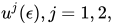Since $\lambda _{1}\neq \lambda _{2}$ for $\epsilon \neq 0$ if $u^{j}(\epsilon ),j=1,2,$ are any normalized eigenvectors belonging to 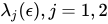$\lambda _{j}(\epsilon ),j=1,2$ respectively then 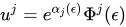$u^{j}=e^{\alpha _{j}(\epsilon )}\Phi ^{j}(\epsilon )$ where $\alpha _{j},j=1,2$ are real for $\epsilon \neq 0.$ It is obviously impossible to define $\alpha _{1}(\epsilon )$ , say, in such a way that $u^{1}(\epsilon )$ tends to a limit as $\epsilon \rightarrow 0,$ because $|u^{1}(\epsilon )|=|\cos(1/\epsilon )|$ has no limit as $\epsilon \rightarrow 0.$

Note in this example that $A_{jk}(\epsilon )$ is not only continuous but also has continuous derivatives of all orders. Rellich draws the following important consequence. << Since in general the individual eigenvectors do not depend continuously on the perturbation parameter even though the operator $A(\epsilon )$ does, it is necessary to work, not with an eigenvector, but rather with the space spanned by all the eigenvectors belonging to the same eigenvalue. >>

Example 2

This example is less nasty that the previous one. Suppose $[K_{0}]$ is the 2x2 identity matrix, any vector is an eigenvector; then $u_{0}=[1,1]^{T}/{\sqrt {2}}$ is one possible eigenvector. But if one makes a small perturbation, such as

$[K]=[K_{0}]+{\begin{bmatrix}\epsilon &0\\0&0\end{bmatrix}}$

Then the eigenvectors are $v_{1}=[1,0]^{T}$ and $v_{2}=[0,1]^{T}$; they are constant with respect to $\epsilon$ so that $\|u_{0}-v_{1}\|$ is constant and does not go to zero.

See also

• Perturbation theory (quantum mechanics)
• Bauer–Fike theorem

Further reading

Books

• Ren-Cang Li (2014). "Matrix Perturbation Theory". In Hogben, Leslie (ed.). Handbook of linear algebra (Second ed.). CRC Press. ISBN 978-1466507289.
• Rellich, F., & Berkowitz, J. (1969). Perturbation theory of eigenvalue problems. CRC Press.{{cite book}}: CS1 maint: multiple names: authors list (link).
• Bhatia, R. (1987). Perturbation bounds for matrix eigenvalues. SIAM.

Report

• Rellich, Franz (1954). Perturbation theory of eigenvalue problems. New-York: Courant Institute of Mathematical Sciences, New-York University.

Journal papers

• Simon, B. (1982). Large orders and summability of eigenvalue perturbation theory: a mathematical overview. International Journal of Quantum Chemistry, 21(1), 3-25.
• Crandall, M. G., & Rabinowitz, P. H. (1973). Bifurcation, perturbation of simple eigenvalues, and linearized stability. Archive for Rational Mechanics and Analysis, 52(2), 161–180.
• Stewart, G. W. (1973). Error and perturbation bounds for subspaces associated with certain eigenvalue problems. SIAM review, 15(4), 727-764.
• Löwdin, P. O. (1962). Studies in perturbation theory. IV. Solution of eigenvalue problem by projection operator formalism. Journal of Mathematical Physics, 3(5), 969–982.